

Research Article
General approach for quantitative description of the Background Voltammograms
1Radioelectronic and Informative-Measurements Techniques Department, Kazan National Research Technical University (KNRTU-KAI),
Kazan, Russia
2Institute of Chemistry, Kazan Federal University (KFU), Kazan, Russia
3Chemistry Department, Bashkir State University (BSU), Ufa, Russia
*Corresponding author: Elza I Maksyutova,
Department of Chemistry,
Bashkir State University (BSU),
Ufa, Russia,
Email: artsid2000@gmail.com
elzesha@gmail.com
Received: October 25, 2017 Accepted: November 27, 2017 Published: December 02, 2017
Citation: : Nigmatullin RR, Budnikov HC, Sidelnikov AV, Maksyutova EI. General approach for quantitative description of the Background Voltammograms. Madridge J Anal Sci Instrum. 2017; 2(1): 47-55. doi: 10.18689/mjai-1000110
Copyright: © 2017 The Author(s). This work is licensed under a Creative Commons Attribution 4.0 International License, which permits unrestricted use, distribution, and reproduction in any medium, provided the original work is properly cited.
Abstract
Based on the hypothesis related to fractal structure of electrode one can develop the
quantitative theory for description of the measured voltammograms (VAGs). We suppose
that at least two percolation channels take part in the process of its formation. One channel
can be associated with the fractal structure of electrodes while the second one can be
related to the heterogeneous structure of the double electric layer. Based on the obtained
fitting function that follows from the suggested theory it becomes possible to differentiate
the state of two measured electrodes (with regeneration or without application of this
procedure). This result obtained directly from the measured data can find a wide application
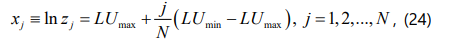
in electrochemistry for analysis of other VAGs, especially in detection of possible traces of
substances that take place in chemical reactions in the vicinity of heterogeneous electrodes.
Keywords: Electrochemistry; Quantitative Fractal Theory; Regenerated/No Regenerated
Electrodes; Self-Similar Voltammograms; Traces Detection.
List of abbreviations: BLC - bell-like curve, DEL - double electric layer, GCE - the glassy
carbon electrode, ECs - the eigen-coordinates method, LLSM - the linear least square
method, PD - potential distribution, VAG(s) - voltammogram(s).
Introduction and Formulation of the Problem
As it is known for detection of the limit of sensitivity of the presence of a substance by
electrochemical methods a researcher uses the series of measurements in the presence of
analyte (i.e. a blank experiment) or the background electrolyte. Detection of this signal
determines the minimal concentration of the electrolyte in the analyzed object [1]. Detection
of this signal gives a possibility (with some value of probability) to extract a useful signal
among random factors (noises) and based on the ratio signal/noise (S/N) to evaluate the
desired limit of detection. This limit can be evaluated in accordance with standard deviation
(dispersion of the background signal) using the ratio 3sbg/b, where b determines the sensor
sensitivity coefficient. The uncontrollable factors (noises) can have different origins. It can be
suppressed by chemical/instrumental methods [2,3] or based on some mathematical
methods, for example, with the help of projection method suggested by chemometrics [4].
The complete elimination of the background is impossible. Especially, it creates a big
problem in interpretation of complex multi-parametric data in the presence of multisensors.
To this problem one can refer, for example, the VAGs associated with electronic “tongue” [5].
For the increasing of electrochemical resolution many methods were suggested and
their descriptions one can find in paper [6]. However, even in the conditions of the wellresolved
peaks, the measured VAGs contain the background current component (for example, capacity current), which strongly distorts the measured
VAG, especially at small electrolyte concentrations. This problem
complicates the data decoding and decreases the sensitivity and
accuracy of the electrochemical analysis in detection of possible
traces of the presence substance. These existing problems are
described in papers [3,6]. The mathematical modeling of the
voltammetric behavior on different types of electrodes is
discussed in [7]. But it is necessary to note that many leading
researches (Compton et al) demonstrate the forms of the VAGs
for electrodes having large surface and for relatively large
concentrations of depolarizator (at large values of the faraday
currents) and, naturally, the “background” problems are skipped
and not discussed properly [7].
In the conditions of multivariate study the synergetic
effects of the present components in formation of the double
electric layer (DEL) strongly distort the measured curves [8,9].
We want to stress also that approach based on the subtraction
of the signals in the systems of the electronic tongue type
becomes useless [10,11].
It is obvious that new approaches for decoding and
mathematical description of the VAGs are necessary. They should
take into account the factors that influence on the dispersion of
the background signals in all possible range of potential created
by the used sensor. In this aspect a certain interest can be referred
to approaches associated with electrochemical behavior of
electroactive particles on different electrodes based on the ideas
of fractal geometry [12-17]. It is well known that electrochemical
activity as response of the electrode varies over its surface. One
can propose some cases of such typical phenomena:
- partially blocked electrode,
- composite electrode (made of composite material with nanoparticles),
- chemically modified electrode (especially with catalytic active particles),
- Screen printed partially blocked electrode with random particles of various forms on the surface.
In all these cases a chaotic distribution of particles is
observed. Partially blocked electrode is used for ordinary case
especially when a macro electrode covered with inert particles
of a material is different to that of the underlying electrode
surface. These particles can block the diffusional paths of the
electroactive species to the electrode surface. To be true, this
conclusion is only correct if both zones of the electrodes -
blocked and exposed - are of macro size. If they are of micronsized
dimensions then the voltammetric response is much
more difficult to predict [7]. This brief review of the present
situation allows formulating the problem that can be
considered in this paper.
The authors suggest an original approach to description
of the real background electrolyte based on the confirmed
real data. This approach based on the fractal theory allows to
describe quantitatively the behavior of the measured VAGs
associated with real electrolyte in two conditions: (a) when the
sensor was regenerated; (b) when the sensor becomes idle
and was not subjected to the regeneration procedure.
For more accurate detection of these different states it
would be desirable to suggest the analytical form of the given
voltammogram (VAG) or the fitting function. Based on the
preliminary results obtained earlier in [18] in this paper we give
some arguments for justification of the desired dependence of
the function J (U). With the help of the eigen-coordinates
method (developed earlier by one of the authors (RRN)) in [19]
we proved that the function J (U) is described by a linear
combination of the power-law exponents with log-periodic
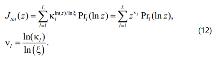
corrections. As it follows from the general theory described
below the desired fitting function based on the fractal structure
of the medium (one can imply the surrounding DEL) and
heterogeneous electrodes themselves can be written as
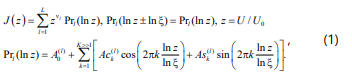
The number of the power-law exponents nl
(l = 1,2,…,L)
for description of the given VAG and the value of the final
mode K should be sufficient for keeping the value of the
relative fitting error less than 5%-7%. The parameter z
coincides with the dimensionless potential Ush/U0 shifted to
positive region (z > 0). The power-law exponents nl
(l = 1,2,…,L) are real but the complex-conjugated parts are appeared
from the log-periodic functions Prl
(lnz). For explanation and
justification of expression (1) chosen as the basic fitting
function one can suggest rather general theory based on idea
of formation of some self-similar percolation channels
connecting the total current under the applied potential. This
theory justifies expression (1) chosen as the fitting function
and naturally explains the appearance of the complexconjugated
power-law exponents.
The content of the paper is organized as follows. In the
second section we describe the experimental details. In the
third chapter we suggest the general theory that explains
expression (1) and its possible modifications. In the fourth
section the desired algorithm for the fitting of the background
currents for different electrodes is described. In the final
section we discuss the obtained results and speculate about
the physical/chemical meaning of the suggested fitting
function.
Experimental
Reagents and the used equipment
All voltammetric measurements were performed with the
help of three-electrode scheme and the usage of voltammetric
analyzer IVA-5 (Yekaterinburg, Russia). The glassy carbon
electrode (GCE) was used as the working electrode. The glassy
carbon pivot and chloride-silver Ag/AgCl (3.5 M KCl) electrode
were used as an auxiliary electrode and comparison electrode,
correspondingly. Voltammetric measurements were
performed in the potential range from 0.0 up to -1.5 V in the
given cycling regime. For the cleaning of the electrode surface
at mechanical regeneration the standard GOI polishing paste
was used.
Voltammetric measurements
In the electrochemical cell 10 ml of the standard solution
of 0.1 M KCl was placed. Each experiment includes the
electrochemical cleaning of the standard GCE during 30 sec at
the applied potential 0.4 V. The cyclic VAGs were registered in
the potential range 0.0 - (-1.5) V with the scanning rate 0.1 V/
sec. All measurements were performed at room temperature
(21-23°C). We obtained two types of VAGs: the first type - the
measured data for electrodes without regeneration (electrodes
were kept in the measured cell during the whole period of
measurements). The second type of VAGs was obtained with
the usage of regeneration procedure, when the surface of
electrodes was polished on the smooth paper by a special GOI
polishing paste having small grains. For verification of stability
of the measurements each cycle of experiment was repeated
100 times.
Results and Discussion
The general theory for quantitative description of the
desired VAG
For explanation and justification of the chosen curve (1)
we put forward the following arguments. Let the function f
(zxn) describes the distribution of the dimensionless potential
z=U/U0 over some fractal electrode. The arising current J (z)
evoked by the applied potential is distributed over percolation
regions and the distribution of these regions has a fractal
(scaling) structure. Mathematically this supposition will be
expressed in the form of the sum
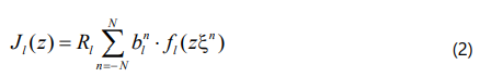
Here the value Rlbln determines the percolation region
that can coincide with volume (dε=3), surface (dε=2) or
conducting line (dε=l). The function
fl(zξn) determines the
distribution function of the potentials that can be specific for
each l-th “channel” of the type (2) that provides the percolation
process of the total current from one electrode to another
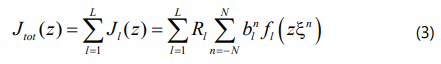
one. For any heterogeneous structure that constitutes a
possible fractal structure of the used electrodes and
percolation regions of the conducting “surrounding”
(including also the DEL) we suppose that all conducting
channels form an additive combination of currents that can
connect two or more electrodes with each other. So, one can
write the following expression for the total current as
We suppose also that the function describing the potential
distribution (PD) for each microscopic current (f1 zξn) has
the following asymptotic behavior at small and large values of
N
For z << 1
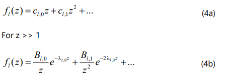
If the values of these functions (f1 zξn) (l = 1,2,…,L) are
small for large and small values of z then one can show [20-
22] that the fractal sum (2) can be reduced to the simplified
functional equation of the type
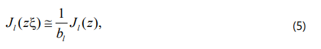
For any combination of parameters bl
, x. It implies that
asymptotic influence of the PD function becomes small 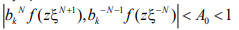 in the ends of a fractal region [20]. The solution of the functional equation (5)
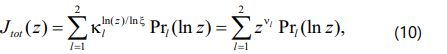
is expressed in the form
in the ends of a fractal region [20]. The solution of the functional equation (5)
is expressed in the form
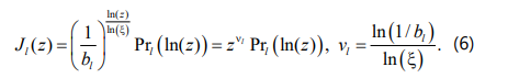
The log-periodic function is defined by expression (1). Let
us suppose that we have at least two “channels” of the type (2)
and the total percolation process is expressed as
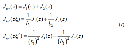
Excluding two channels J1,2(z) from the first two lines and
inserting them to the final line we obtain the following
functional equation for the total current
where
In paper [22] it was shown that this functional equation has the following solution
Using the mathematical induction method one can show that this result can be generalized for �L� conducting channels. For this case we obtain
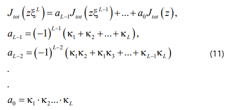
As for the case L = 2 the desired roots kl
are related to the
scaling parameters bl
by means of simple relationships kl
= 1/
bl
(l = 1,2,…,L). The solution of the functional equation (11) has
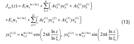
the following form [22]
In order to minimize the number of the fitting parameters
we consider in detail the case L=2. The fitting function that
can describe the desired VAG can be rewritten in the form
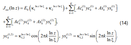
In order to reduce number of the fitting parameters in
expression (13) we suppose that two channels involved in the
percolation process have equal contributions (K = Q). For this
case the function (13) admits further simplification and finally
for the case L=2 we obtain the following fitting function
In the next section we show how to calculate the desired
parameters k1,2 and nonlinear fitting parameters as lnx and K.
Obviously, the common scaling parameter lnx that enters in
the general expressions (12-14) should be interpreted in the
mean value sense. This simplification and selection the
common value for all possible channels is explained in the
Mathematical Appendix.
Some peculiarities of the fitting of expression (14) to real data
In this fitting function we have 4 nonlinear parameters
k1,2, lnx and K. Other fitting parameters as E0, Ack(1,2), Ask(1,2) equaled to 4K+1 are found by the LLSM. The value of the
desired x is located in the interval
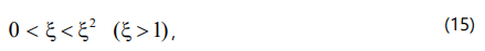
While the final value of K is calculated from the condition
that the value of the fitting error should not exceed 5-7% for
simple case. This value is calculated as
Where the fitting function  coincides with the simplified expression (14), the fitting vector
  and y(z) coincides with mean measurement VAG. The
evaluation of this mean measurement from the given set of
data is explained in the next section. We should stress here
that in the case of negative values of k that can enter in the
fitting function (14) the corresponding expression should be
replaced as
and y(z) coincides with mean measurement VAG. The
evaluation of this mean measurement from the given set of
data is explained in the next section. We should stress here
that in the case of negative values of k that can enter in the
fitting function (14) the corresponding expression should be
replaced as
The Description of the Data Processing Procedure
The basic problem that can be solved in the frame of the
suggested theory is formulated as follows: is it possible “to
notice” the difference between non-regenerated and
regenerated electrodes and express their differences
quantitatively? All treatment procedure can be divided on
three basic stages that can be recommended as a common
procedure for all similar measurements, as well.
Stage 1. Reduction to Three Mean Measurements.
We show this procedure for electrode without
regeneration. It is also explained by the figures given below.
The same procedure will be applied to analysis of the VAGs
with regeneration. The initial hysteresis (cycle) of the measured
function J(U) for electrodes without regeneration is shown in
Fig.1. Accordingly, the VAGs corresponding to the regeneration
procedure were shown in Fig.2.
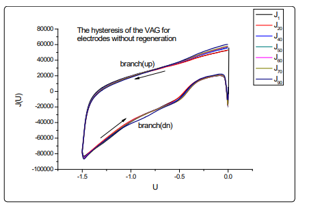
For further analysis we divide the hysteresis on two
branches (up and down) correspondingly and consider them
separately.
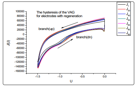
One can notice visually the difference between these
VAGs but the basic aim is to find the fitting function for these
curves and then “read” and compare them quantitatively.
The basic aim of this stage is to receive the averaged
VAGs that can be prepared for the fitting procedure with the
function (14). In order to realize the correct averaging
procedure we consider the branches (up and down) forming
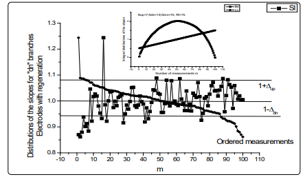
the initial hysteresis separately. We consider the distribution
of the slopes with respect to mean measurement
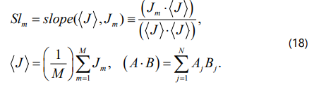
Here M=100 coincides with the total number of
measurements for the given background. The sufficiently
large of repetitions (50 < M < 100) of the same electrochemical
background are necessary for analysis of statistical peculiarities
and the influence of external conditions that will take place
during the whole experiment. The parenthesis in (18)
determines the scalar product between two functions having
j=1,2,…,N measured data points. If we construct the plot Slm
with respect to successive measurement m and then rearrange
all measurements in the descending order SL1 > SL2 > … > SLM,
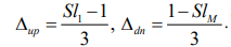
then all measurements can be divided in three groups. The
“up” group has the slopes located in the interval (1+Dup, SL1);
the mean group (denoted by “mn”) with the slopes in (1-Ddn,
1+Dup); the down group (denoted by “dn”) with the slopes in
(1-Ddn, SLM). The values Dup,dn are chosen for each set of the
VAG measurements separately. In our case we chose the
conventional “3sigma” criterion and put
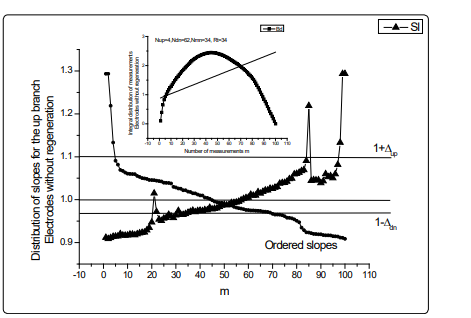
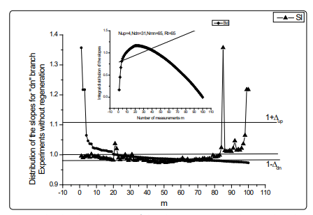
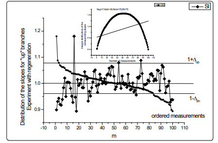
 . This curve has a great importance
and reflects the quality of the realized successive measurements
and the used equipment. Different cases for 4 different
branches and two types of electrodes are shown on Figs. 3(a,
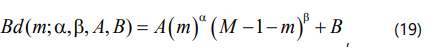
b, c, d), correspondingly. The bell-like curve (BLC) (that can be
fitted with the help of four fitting parameters α, β, A, B) is
obtained after elimination of the corresponding mean value
and subsequent integration can be described by the non-normalized beta-function
. This curve has a great importance
and reflects the quality of the realized successive measurements
and the used equipment. Different cases for 4 different
branches and two types of electrodes are shown on Figs. 3(a,
b, c, d), correspondingly. The bell-like curve (BLC) (that can be
fitted with the help of four fitting parameters α, β, A, B) is
obtained after elimination of the corresponding mean value
and subsequent integration can be described by the non-normalized beta-function
and reflects the quality of the realized measurements. This
presentation is very convenient and contains additional
information about the process of measurement that before
was not taken into account. The straight line (it can have a
slope not coinciding with horizontal line) divides all
measurements in three groups: (a) the beginning point of a
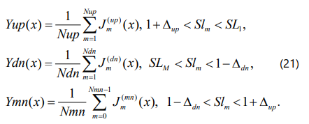
BLC up to the first intersection point determines the number
Nup of measurements (Jm(up)(x) (m=1,2,…, Nup) entering in
the “up” group and is characterized by the mean Yup(x) curve;
(b) the region between the two intersection points determines
the number Nmn of measurements (Jm(mn)(x) (m=1,2,…,Nmn)
in the “mn” group with slope close to one and characterized
by the set of measurements forming the mean curve Ymn(x)
and, finally, (c) the rest of the measurements Ndn in the “dn”
group is covered by the curve Ydn(x). If the number of
measurements Nmn > Nup+Ndn then this cycle of
measurements is characterized as “good” (stable), in the case
when Nmn»Ndn»Nup the measurements (and the
corresponding equipment) are characterized as “acceptable”,
and the case when Nmn < Nup+ Ndn is characterized as “bad”
(very unstable). Quantitatively, all three cases can be
characterized by the ratio
In the last expression (4), M determines the total number
of measurements. Based on this ratio one can determine
easily three classes of measurements: “good” when 60% < Rt
< 100%, “acceptable” when 30% < Rt < 60%, and “bad” when
0 < Rt < 30%. This preliminary analysis is supported by Figs.
3(a, b, c, d) for four branches of the measurements with/
without electrodes regeneration.
So, if this clusterization will be realized then instead of
100 initial measurements we have approximately
Here the function Slm determines the slopes located in the
descending order and the parameters Dup,dn associated with
the value of the confidence interval is selected for each
specific set of measurements separately. After realization of
this useful procedure one can fit only the mean function
Ymn(x). Other two functions Yup(x) and Ydn(x) become
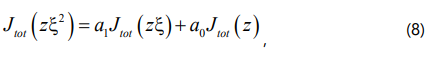
strongly-correlated and can be associated with two close
curves in accordance with expression (8)
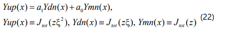
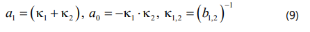
This simple observation allows us to find the unknown
constants a1,0 from the LLSM and calculated the desired roots
from the quadratic equation
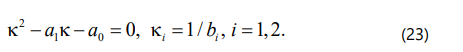
Equation (23) allows restoring also the scaling parameters
bi
entering to the percolation channel (2). In equation (22) we
have two independent variables x and z. It is necessary to
choose the common scale that could be acceptable for the
realization of the fitting procedure. If we choose the following
values for the down (dn) VAG branch as LUmax = ln(Umin/ -1)
with U0=-1 and LUmin = ln(10-2) and for the “up” branch the
variable LUup=-LUdn then in this scale
corresponding VAGs remains invariant relatively the chosen number of points. So, this scale as the most convenient is chosen for the fitting purposes.
Stage 2. The Fitting of the Mean Curves Ymn(lnz) to the
Function (14)
For realization of the desired fit we normalize these curves
to the interval [0,1] that cannot change essentially the essence
of the applied approach. As it has been mentioned above, we
chose the logarithmic scale (24) where the corresponding
VAGs do not change their form. The normalized mean curve
for two branches and two experimental situations (without
and with electrodes regeneration) are calculates as
We take the small value of the e = 10-6. These two simple
linear transformations realized for the mean curves Ymn(x) allow
avoiding some large values of the fitting parameters and uncertainties related the taking of the natural logarithm from
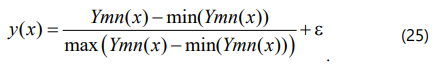
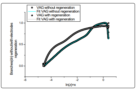
zero. The final fit of the normalized curves for all four branches
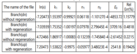
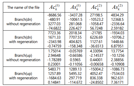
are depicted on Figs.4 (a,b), correspondingly. The additional
fitting parameters (lnx, k1,2, n1,2) and the distributions of the
amplitudes Ack(1,2), Ask(1,2) (k=1,2,…,K=4) entering into
expression (14) for these four normalized branches are collected
in Tables 1, 2, correspondingly. So, this theory helps to restore
the fractal parameters and partly its discrete structure that
characterize the percolation structure of the conducting channels.
Stage 3. Reduction to Three Incident Points as the Test of
a Possible Self-Similarity
In this subsection we want to suggest a test for detection of
self-similar curves that form the measured VAG. Let us choose
some interval [x0, xk-1] containing a set of k data points {(x0, y0),
… , (xk-1, yk-1) K=0,1,…,k-1}. One can reduce this information into
three incident points if the first point is associated with the mean
value of the amplitudes and the other two points are associated
to their maximal and minimal values, correspondingly. So, this
selection represents the simplest reduction of the given set of k
randomly selected points to three characteristic points
p1=mean{y0, … , yk-1}, p2=max{y0, … , yk-1}, p3=min{yk-1, … , yk-1}. If
in the result of this reduction procedure we obtain the curve
similar to the initial one then one conclude that obtained three
curves are self-similar to the initial curve. This procedure helps
to decrease the number of initial points and consider the
reduced curves distributed over on the set of “fat” points. R =
[N/L], r = 0,1,…,R-1. Here the symbol [..] defines the integer part
of the ratio N/K, where N is the total number of points and K is
the length of the chosen “cloud” of points. The result of
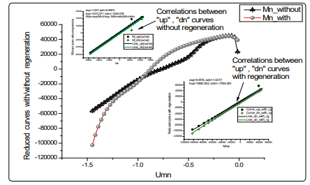
reduction of two “down” initial VAGs and corresponding to
electrodes with/without regeneration are shown in Figs. 5(a,b).
For R=50, L=24 the self-similarity property is clearly noticeable.
The same result is obtained for two self-similar curves
corresponding to “up” branches and thereby it is not shown.
This simple test serves as an additional argument for selection
of the fitting model (14) described above.

Conclusion
May be this theory is not complete but it reflects the
influence of existing fractal structure of the measured electrodes
and conducting media that take place during the electrochemical
process. We believe that this theory can find its wide application
for quantitative description of a various VAGs. In particular, in
solutions of electroanalysis problems associated with in
detection of possible traces of the solute substances, when the
peaks of oxidation\restoration potentials are close to each
other. This phenomenon is observed in analysis of VAGs
associated with optically active compounds as enantiomers,
having practical importance in medicine. From practical point of
view, the suggested quantitative method one can apply for
evaluation of the effectiveness of the medical drug and identify
one enantiomer (the micro component of the medical drag with
negative reaction to the human′s body) and in its abundance,
when it has a positive influence. In this case, the total background
current will coincide with current of the given solute mixed with
current belonging to macro-component. The detection of the
micro-component current one can evaluate quantitatively
analyzing, in turn, the measured VAG based on the approach
suggested above. But the additional and justified arguments
tested on a wide experimental material need a further research.
Mathematical Appendix
In this Appendix we want to justify the common selection
of the scaling parameter x that enters in the general fitting
formula (12). Let us suppose that instead of the scaling factor
xn we have the product ξ1ξ2...ξn generated by the random structure of the percolation cluster. We suppose also that these random scaling factors have small deviations relatively
the mean value , 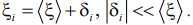 If we put these
factors into the product we obtain
If we put these
factors into the product we obtain
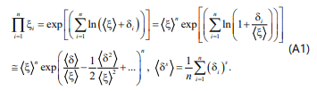
This useful relationship shows that it is possible to replace
the set of the random scaling parameters by one averaged
parameter in accordance with the relationship
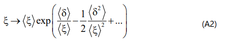
Therefore in the main text we imply this parameter in the averaged sense, which is evaluated with the help of the fitting procedure
Acknowledgement
This work was supported by Russian Science Foundation, project No16-13-10257.
References
- Eksperiandova LP, Belikov KN, Khimchenko SV, Blank TA. Once again about determination and detection limits. J. Anal. Chem. 2010; 65(3): 223- 228. doi: 10.1134/S1061934810030020
- Otto M. Analytische Chemi. Weinheim: Wiley-VCH; Fourth edition, 2011.Scholz F (Ed.) Electroanalytical Methods, Guide to Experiments and Applications. Springer-Verlag Berlin Heidelberg. 2002.Pomerantsev AL. Chemometrics in Excel. New York: Wiley Online Library. 2014; doi: 10.1002/9781118873212Winquist F, Wide P, Lundstrom L. An electronic tongue based on voltammetry. Anal. Chim. Acta. 1997; 357(1-2): 21-31. doi: 10.1016/S0003-2670(97)00498-4Henze G. Polarographie und Voltammetrie. Springer-Verlag Berlin Heidelberg. 2001.Compton RG, Banks CE. Understanding voltammetry: Second edition. Imperial College Press. 2011.Hamann CH, Vielstich W. Elektrochemie, Bd. I u. II aus der Reihe „taschentext“.Weinheim: Verlag Chemie. 1975.Schwabe K. Physikalische Chemie, Bd. 2, Elektrochemie. Akademie-Verlag Berlin. 1986.Winquist F. Voltammetric electronic tongues - basic principles and applications. Microchim. Acta. 2008; 163(1-2): 3-10. doi: 10.1007/s00604-007-0929-2Winquist F, Olsson J, Eriksson M. Multicomponent analysis of drinking water by a voltammetric electronic tongue. Anal. Chim. Acta. 2011; 683(2): 192-197. doi: 10.1016/j.aca.2010.10.027.Ruiz GA, Felice CJ. Electrochemical-fractal model versus randles model: A discussion about diffusion process. Int. J. Electrochem. Sci. 2015; 10(10): 8484-8496Anastopoulos AG, Bozatzidis AI. Detection of the fractal character of compact adsorbed layers by the dropping mercury electrode. Electrochim. Acta. 2009; 54(16): 4099-4104. doi: 10.1016/j.electacta.2009.02.042Felice CJ, Ruiz GA. Differential equation of a fractal electrode-electrolyte interface. Chaos, Solitons and Fractals. 2016; 84: 81-87. doi: 10.1016/j. chaos.2016.01.003Fernández-Martínez M, Nowak M, Sánchez-Granero MA. Counterexamples in theory of fractal dimension for fractal structures. Chaos, Solitons and Fractals. 2016; 89: 210-223. doi: 10.1016/j.chaos.2015.10.032Mayrhofer-Reinhartshuber M, Ahamme H. Pyramidal fractal dimension for high resolution images.Chaos. 2016; 26 (7): 1-7. doi: 10.1063/1.4958709Kant PR. General Theory for Pulse Voltammetric Techniques on Rough and Finite Fractal Electrodes for Reversible Redox System with Unequal Diffusivities. Electrochim. Acta. 2016; 194: 283-291. doi: 10.1016/j. electacta.2016.02.039Nigmatullin RR, Budnikov HC, Sidelnikov AV. New Approach for Voltammetry Near Limit of Detection: Integrated Voltammograms and Reduction of Measurements to an “Ideal” Experiment. Electroanalysis. 2015; 27(6): 1416-1426. doi: 10.1002/elan.201400735Nigmatullin RR. Recognition of nonextensive statistical distributions by the eigencoordinates method. Physica A. 2000; 285(3-4): 547-565. doi: 10.1016/S0378-4371(00)00237-5Nigmatullin RR, Le Mehaute A. Is there geometrical/physical meaning of the fractional integral with complex exponent? J. Non-Cryst. Solids. 2005; 351(33-36): 2888-2899. doi: 10.1016/j.jnoncrysol.2005.05.035Nigmatullin RR, Machado JT, Menezes R. Self-similarity principle: the reduced description of randomness. Central European Journal of Physics. 2013; 11(6): 724-739. doi: 10.2478/s11534-013-0181-9Nigmatullin RR, Baleanu D. New relationships connecting a class of fractal objects and fractional integrals in space. Fractional Calculus and Applied Analysis. 2013; 16(4): 911-936. doi: 10.2478/s13540-013-0056-1
