Abstract

Understanding the mechanical controls on shear strength decrease due to preexisting weakness is a fundamental problem in tectonic studies. In this study, by applying reactivation tendency analysis theory, a theoretical framework and defined Shear-strength Coefficient (f_d) are developed for evaluating the shear-strength decrease and anisotropies due to the presence of preexisting weakness(es). The proposed study managed to overcome the restrictions of previous studies assumption that a pre-existing weakness plane contains the intermediate stress (σ₂ ) and vertical or horizontal orientations of principal stresses (Andersonian stress state). A new graphical technique (Mohr-space) was utilized to predict the shear-strength decrease and anisotropies caused by preexisting weakness(es). The Mohr-space technique made easier to visualize the state of stress and results of shear strength changes and able to build the quantitative and intuitive relationship between Shear-strength Coefficient (f_d) and weakness relativeorientation(θʼ,φ’), weakness mechanical properties (C_w and µ_w) and relative in any uniform tri-axial stress state.. In this study, Shear-strength decrease and anisotropies of a rock sample are evaluated theoretically, and shear strength properties and deformation characteristics of a geological body with multiple pre-existing weaknesses are analyzed and predicted.

Key words: Shear strength; preexisting weakness; reactivation tendency; Mohr-space; sandbox experiment.

Introduction

It is well documented that pre-existing weaknesses (fracture planes or faults, layering, fabrics etc.) can lead to decrease of shear strength and strength anisotropies [1-3], and the potential strength anisotropy created by pre-existing weakness is considerable [4]. Ranalli (1990) [5] proposed a unified quantitative model to evaluate strength anisotropies by the pre-existing weakness in terms of the three tectonic faulting regimes when the weakness plane contains the intermediate stress (σ₂ ). However, to our knowledge strength anisotropies evaluation with pre-existing weakness is limited to two-dimensional cases (weakness plane containing σ₂ ) before slip-tendency theory was proposed [6]. However, strength anisotropies evaluation with slip-tendency [7] is confined to the qualitative analysis only. In addition, there is also some limitation in slip-tendency theory, i.e. the principal stresses are oriented either vertically or horizontally, and the cohesive strength of all preexisting weakness is neglected [6]. However, principal stress direction may depart significantly from vertical and horizontal with depth in the upper crust [8-9]. Furthermore, some weakness zones may possess cohesive strength, particularly in cemented faults, and properties of weaknesses may vary [4]. For a example, Sibson (1974) [10] showed that cementation of a fault zone can create 1.0-MPa cohesive strength or more. In this study, Shear-strength Coefficient (f_d) is defined, and Reactivation Tendency analysis theory [11], and Mohr-space [12] are applied to evaluate strength decrease and anisotropies due to the presence of pre-existing weakness(es) with arbitrary azimuth in any uniform tri-axial stress state. Strength decrease and anisotropies caused by weakness may be intuitively simplified and quantitatively analyzed and evaluated with Mohr space.

Mohr-space, pole (σ_n, τ_n) of any oriented plane in tri-axial stress state

Mohr diagrams, which was introduced by Otto Mohr (1882), is one of the most used and useful tools in structural geology [13], and has been used extensively in mechanical problems, such as stress analysis, failure envelopes, fractures opening and reactivation [14] [15] [16] [17]. Although real three-dimensional Mohr diagrams do exist for any tri-axial stress state [13], Mohr-diagram is usually considered to be two-dimensional [13], which is well known as Mohr-circles. Mohr-cyclides, which can be used to represent any second rank tensor (including stress tensor) was introduced by Coelho and Passchier (2008) [13]. However, the stress components (σ_n , τ_n ) of any given plane are the most important, and the general diagrams of Mohr-cyclides are not so convenient to be used and prepared. In contrast, the Mohr space, which was proposed by Tong and Yin (2011) [11] can be used to express the normal stress and shear stress of a plane with an arbitrary azimuth in an arbitrary three-dimensional stress state.

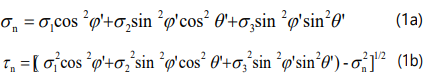
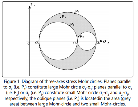
In any given stress state, the pole (σ_n , τ_n ) of any plane (i.e. pre-existing weakness plane, defined by dip direction θ and dip angle φ) is either located on the three Mohr-circles (i.e. P₁ on large Mohr circle σ₁ -σ₃ , P₂ and P₃ on small Mohr circles σ₁ - σ₂ and σ₂ -σ₃ respectively, Figure 1) or in the area (grey area in Figure 1) between large Mohr-circle and two small Mohrcircles(i.e. P₄ in Figure 2) in σ_n -τ_n coordinate system [2,18]. There is one to one correspondence relationship between any plane and its pole (σ_n , τ_n ) in σ_n -τ_n coordinate system. This space (i.e. the three Mohr-circles and the area between them) is called Mohr-space [11]. With the contour lines (pink and green dotted lines in Figure 2) of plane angles (pseudo-dip direction θ’ and pseudo-dip angle φ’, θ>= α> +90 °, where α> is the angle between the plane and the intersection line of the plane and σ₂ -σ₃ plane; φ> the angle between the plane and σ₂ -σ₃ plane), the pole of the plane can be found in the Mohrspace. The relationship between θ>, φ>, θ, and φ can be determined with transformation of coordinates [11], and the contour lines of angles can be compiled with equation (1) [11].

Coordination definition and transformation can be seen in Tong and Yin (2011) [11].

Thus, by applying Mohr-space, normal stress (σ_n ) and shear stress (τ_n ) of any plane can be conveniently and intuitively determined, and the changes of normal and shear stresses with plane relative-orientation (θ´,φ>) can be easily analyzed.

Reactivation Tendency Factor and its expressions in Mohr-space

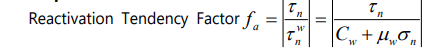
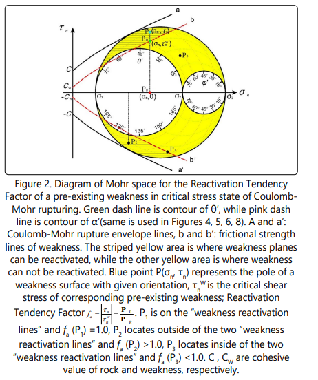
(where τ_n , σ_n are shear and normal stresses on the weakness plane, respectively; τ_n^w is the corresponding rupture shear strength; C_w, and µ_w are cohesiveness and frictional coefficient of weakness plane, respectively), which is extended from Sliptendency [6] and is used to evaluate the reactivation likelihood of pre-existing weakness, is proposed by Tong and Yin[11] (2011). Reactivation Tendency Factor (f_a ) is determined by its relative-orientation (θ´,φ´), mechanical properties (C_w, µ_w ) of the weak plane, and the stress tensor. f_a =1.0 shows that the pre-existing weakness is in critical state of reactivation; when f_a <1, it has reactivated and when f_a >1, it is in a stable state. The weaknesses, which f_a ≥1.0 in the critical stress state of Coulomb rupture, will reactivate one by one in progressive deformation according to their f_a value order.

Applying Mohr-space, f_a can be intuitively expressed accordingto the following steps. (1) The lines τ_n^w=± (C_w + µ_wσ_n ) are two symmetrical straight lines (when µ_w is a constant)or curved lines(b and b´ in Figure 2, when µ_w is variable) in σ_n -τ_n coordinate system, which were called “weakness reactivation lines” [19] or “shear strength line of weakness ” [11], where (0, C_w ) is the starting point, µ_w is the slope of the line. If C_w = 0 (weakness without cohesion), the line cross the point of origin. (2) The pole (σ_n , τ_n ) of a weakness plane (P in Figure 2) can be easily plotted in Mohr-space according to its relative-orientation (θ´and φ´) and its σ_n , τ_n w can be intuitively determined (Figure 2). As such, f_a (τ_n /τ_n w) of the weakness plane can be easily and intuitively determined (PP₀ /PP_R in Figure 2). (3) When the pole of the weakness plane is on its “weakness reactivation line” (P₁ in Figure 2), f_a =1.0 and the pre-existing weakness is in the critical state of reactivation. However, when the pole is located outside the two “weakness reactivation lines” (striped yellow area in Figure 2, i.e. P₂ ), f_a >1.0 and the weakness plane has reactivated. When the pole is located inside the two weakness reactivation lines (yellow area without stripes in Figure 2, i.e. P₃ ), f_a<1 indicating that the plane is in a stable state.

The definition of Shear-strength coefficient and its relationship to Reactivation Tendency Factor of pre-existing weakness

As a weakness plane may be reactivated when stress is below Coulomb rupturing stress state, a pre-existing weakness will lead to decrease in shear strength [1] [2] [7]. However, the weakness with f_a <1.0 will not reactivate at critical stress of Coulomb rupture [11] according to Reactivation Tendency analysis theory. This means that not all weakness planes will lead to decrease in shear strength. －Therefore, in the following shear strength analysis, we only consider weaknesses with f_a≥1.0.

Consider a weakness plane (P_w) with a normal n and its reactivation tendency factor f_a ≥1.0 at critical uniform stress state (σ₁ , σ₂ and σ₃ ) of Coulomb rupture (Figure 3). P_w has been reactivated at critical stress state of Coulomb rupture [11], and its pole in Mohr-space is (σ_n , τ_n ) (Point A in Figure 3). With the same normal stress σ_n , P_w will be at critical state of reactivation when its shear stress is τ_n^w (Point B in Figure 3, σ´1 , σ´2 and σ´3 are the three principal stresses) and τ_n^w<τ_n . The large Mohr circle (σ´1 -σ´3 circle) of critical stress state of weakness reactivation is smaller than the σ₁ -σ₃ Mohr circle of critical stress state of Coulomb rupture (Figure 3), that means σ´1 - σ´3 < σ₁ - σ₃ . Thus, in Mohr-space (Figure 3), it is very easy to understand that a weaknesswith f_a >1.0will lead to decrease in shear strength.

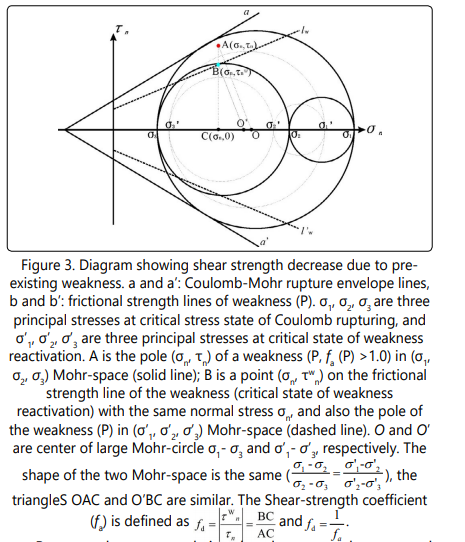
Because shear strength is related to normal stress and increases with increasing of normal stress, relative instead of absolute shear strength is more useful to consider.In order to quantitatively evaluate the shear strength decrease due to the existence of a weakness, we define the parameter f_d called Shear-strength coefficient (f_d = τ_n^w /τ_n , where τ_n^w is the critical shear stress of weakness reactivation, τ_n is the shear stress on the same plane with the same normal stress σ_n at critical stress state of Coulomb rupture (σ₁ , σ₂ and σ₃ stress state in Figure 3)). It is easy to understand that the smaller Shear-strength coefficient (f_d ) is the larger decrease will be in shear strength.

When f_a ≥1.0, τ_n^w can never be greater than τ_n (as stress will drop down when weakness reactivates according to Reactivation Tendency analysis theory [20] [21]. Furthermore, when f_a ≤ 1.0, which means that weakness will not be reactivated at critical stress state of Coulomb rupture and will not lead to shear strength decrease(i.e., f_d=1.0). Therefore, shear-strength coefficient can never be greater than 1.0 (f_d ≤ 1.0).

It is easy to find the following relationship between f_d and Reactivation Tendency Factor (f_a ) at critical stress state of Coulomb rupturing according to the definition of shearstrength coefficient and Reactivation Tendency analysis theory [11]

The relationship between Shear-strength Coefficient (f_d ) and the ratio of Differential stress can be derived at Coulomb rupture ((σ₁ - σ₃ ) C =σ₁ - σ₃ in Figure 3) and at critical state of weakness reactivation ((σ₁ - σ₃ ) W =σ₁ ´- σ₃ ´ in Figure 3) according to the definition of Shear-strength Coefficient and using Mohr-space, and it means that f_d = (σ₁ - σ₃ )_W / (σ₁ - σ₃ )_C. As the relative position of the weakness pole in (σ₁ , σ₂ , σ₃ )-Mohr-space (point A) and in (σ₁ ´, σ₂ ´, σ₃ ´)-Mohr-space (point B) is the same, OA/OB is equal to the ratio of radius of the two big Mohr circle ( 2 σ₁ −σ 3 and 2 σ₁ ´−σ 3´), which means that OA/OB = (σ₁ - σ₃ )/(σ₁ ´- σ₃ ´) = (σ₁ - σ₃ ) C/ (σ₁ - σ₃ ) W. While two triangles AOC and BO´C are similar, as a result, BC /AC =OB /OA and f_d =τ_n w /τ_n = BC /AC = OB / OA = (σ₁ - σ₃ ) C/ (σ₁ - σ₃ ) W, which means that f_d = (σ₁ - σ₃ ) C/ (σ₁ - σ₃ ) W when f_a ≥1.0. So, f_d (1/ f a ) is related to weakness orientation (θ´and φ´), mechanical properties (C_w, µ_w ) and the stress tensor according to Reactivation Tendency analysis theory [11], and it can be quantitatively calculated using equations 1 and 2. Since f_d is related to weakness relative-orientation, weakness can lead to shear-strength anisotropies.

Analysis of shear strength affection factors due to pre-existing weakness(es)

Shear-strength coefficient (f_d) is used to discuss how the related factors (mechanical properties and orientation of weakness, and ) affect shear strength due to preexisting weakness in triaxial stress state. As f_d = 1/f_a , and fa can be intuitively and conveniently expressed in Mohr-space, Mohrspace is applied to do these analysis.

The relationship between f_d and weakness relativeorientation (θ´,φ´)

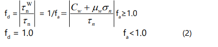
It is easy to see that when θ´=90°, and φ´ =±φ´0 = ± (45°+0.5arctg (µ_w) (φ´0 is usually about 60°) (points A and A´ in Figure 4), f_a reaches the highest value, whereas f_d reaches the smallest value (Figure 4). Therefore, (90°, ± φ´0 ) (two points) are the two weakest relative-orientation of the weakness plane(s). As θ´ decreases from 90°, and φ´ deviates from φ´0 , f_d will increase. In Mohr-space (Figure 4), the points of intersection between “weakness reactivation lines” and Mohr circles are demarcation points of weakness reactivation (B1 , B2 and B´1 , B´2 on σ₁ -σ₃ large Mohr circle, C1 , C2 and C´1 , C´2 on σ₂ -σ₃ small Mohr circle, Figure 4). The corresponding φ´ of B1 , B2 , B´1 and B´2 is φ´1 , φ´2 , φ´1 , φ´2 , and the corresponding θ´ of C1 , C2 and C´1 , C´2 is θ´1 , θ´2 , (180° - θ´1 ) and (180° -θ´2 ) respectively. It is easy to find that when φ´<φ´1 or φ´> φ´2 , or θ´<θ´1 or θ´2 <θ´<180°-θ´2 or θ´>180°-θ´1 , the weakness will all locate inside the two weakness reactivation lines (grey area in Figure 4) and f_a will always <1.0, which means there exist critical angle φ´1 , φ´2 for φ´ and θ´1 ,θ´2 and (180° - θ´1 ),(180° -θ´2 ) for θ´, when φ´<φ´1 or φ´> φ´2 , or θ´<θ´1 or θ´2 <θ´<180°-θ´2 or θ´>180°-θ´1 , fa will always <1.0 and the weakness cannot reactivate and will not lead shear strength decrease (f_d = 1.0).

Point A and A´ (Figure 4) are two Coulomb rupture points, and f_d of the same oriented weakness plane is the lowest. Weakness plane with low f_d value concentrates around point A (or A´) in the yellow area of Figure 4(θ´=90°~75° and φ´=φ´0 ± 15°). Change of f_d shows that weakness relative-orientation is the predominant factor which leads to shear strength anisotropies. It is noteworthy tounderline that (θ´, φ´) of weakness is determined jointly by orientations of weakness and three axes of principal stresses.

The relationship between f_d and weakness mechanical properties (C_w and µ_w)

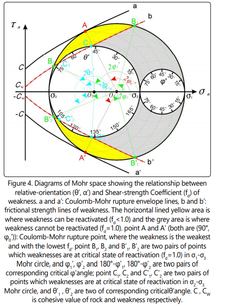
In Mohr-space (Figure 5), it is easy to find that the change of mechanical property of a weakness plane (C_w and µ_w) will cause the change of the position (determined by C_w) and the slope (determined by µ_w) of weakness reactivation lines. It is easy to understand that f_d will decrease with decreasing of C_w and µ_w.

Weakness mechanical properties are the predominant factors which lead to shear strength decrease. For example, low friction coefficient (µ_w< 0.2 [22]) and no cohesion along the weakness may lead to more than 90% shear strength decrease (f_d< 0.1).

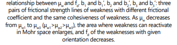
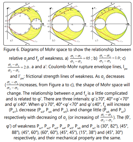
The relationship between f_d and relative value of σ₂

Shear strength is also related to relative value of [7]. However, our analysis in Mohr-space provided intuitive results which are easy to follow. It is easy to see that relative determines the shape of Mohr-space (Fig. 6). The relationship between and f_d is complicated and depends on θ´ and φ´, particularly φ´(Fig. 6). In general, φ´ can be divided into 3 intervals: φ´≥70°, 40°<φ´<70°, and φ´≤40°. When φ´≥70°f_d will increase (P_w1 in Figure 6). When 40°<φ´<70°, f d decreases a little (P_w3, P_w4 and P_w5 in Figure 6), and when φ´≤40°,f_d changes little (P_w6 and P_w7 in Figure 6). These three cases are valid whenσ₂ decrease(or increases, Fig. 6). As such, the change of σ₂ should not be ignored in shear strength analysis in the presence of pre-existing weakness. However, when φ´≥70° or φ´≤40° (particularly when φ´≤40°), most of the weaknesses usually cannot be reactivated at critical stress state of Coulomb rupturing and thus doesnot lead shear-stress decrease (f_d = 1.0). As a result, the effect of relative σ₂ is most prominant only in the interval 40°<φ´<70°; under normal circumstances, f_d will decrease a little with decreasing σ₂ (Fig. 6).

Mechanical properties and relative-orientation, which are the governing factors of shear strength decrease and strength anisotropies, respectively, are internal factors, while is an external factor and not so important according to the above analysis,. When the relative-orientation (θ´, φ´) and mechanical properties (C_w, µ_w ) of pre-existing weakness, and are given, the Shear-strength Coefficient can be quantitatively evaluated in Mohr-space.

Shear strength evaluation for rock samples and geological bodies: theoretical analysis and verification

There are many kinds of pre-existing weakness, such as faults, geologic contacts, bedding and foliation that affect shear strength [23] [24] [25]. Based on their structure, Morley (2002) [26] divided weaknesses into two types: “discrete” and “pervasive”. Based on the value of cohesive strength, Tong and Yin (2011) [11] divide weaknesses into “strong weakness” (with relatively large cohesive strength, such as bedding, foliation etc.) and “weak weakness” (with relatively small or zero cohesive strength (i.e. ignorable), such as faults, fracture planes etc.). “Discrete” weakness is usually a “weak weakness”, and “pervasive” weakness probably is a “strong weakness”. We will evaluate the effect of “strong weakness” and “weak weakness” on shear strength in rock samples, and analyze deformation sequences with multiple pre-existing weaknesses in geological bodies.

Rock samples

“Pervasive” weaknesses (or “strong weakness”, bedding in sedimentary rocks, foliation in metamorphic rocks) do exist in rocks. There may also exist“pervasive” weaknesses in magmatic rocks with ductile deformation or flow foliation. In homogeneous-looking rock samples there may exist “pervasive” (particularly in sedimentary or metamorphic rocks) and /or “discrete” weaknesses (“weak weakness”, internal small or micro-fracture) leading to shear strength anisotropies. In order to quantitatively evaluate shear strength decrease and anisotropies of rock samples with “pervasive” or “discrete” weakness, the situations of ①C_w =0.5C, 0.33C and 0.2C for “pervasive”weakness, and C_w =0 for “discrete” weakness, and ② = 0.5, 1.0 and 2.0 are considered (let µ_w = μ = 0.6, C = 20MPa). Applying Mohr-space, the calculated values of Shear-strength Coefficient can be seen in Table 1. For other C values, the result is completely the same, while the result will change a little bit as μ ( µ_w ) changes (if µ_w = μ ). However, if µ_w changes while μ isconstant, f_d will change proportionally with µ_w .The results show thata “discrete” weakness may lead to more than 80% maximum drop of shear strength, while “pervasive” weakness usually leads to 20-60% maximum shear strength decrease for rock samples.

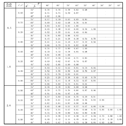
Table 1. Shear-strength Coefficient (f_d ) value in different value of C_W,relative σ₂ , θ´ and φ´

Haimson and Rudnicki (2010) [27] conducted true tri-axial compression tests on siltstone samples, and showed that shear strength is related to σ₂ . Although the orientation of siltstone bedding is not mentioned in the paper, we speculate that the shear strength change is caused by “pervasive” weakness (siltstone bedding). If bedding does not lead to mechanical anisotropy (i.e. when it is mechanically homogeneous), shear strength will not change with σ₂ . The tri-axial compression tests of Haimson and Rudnicki (2010) [28] may be the verification for the above theoretical analysis of dependece of shearstrength on σ₂ . Naturally, availability of more experiment data is needed.

In the presence of multiple pre-existing weaknesses in a rock sample, each weakness has its own Shear-strength Coefficient. The overall Shear-strength Coefficient is determined by and is equal to that of the weakest weakness, where the Shear-strength Coefficient is the smallest, if interactions of weaknesses are ignored.

Geological bodies and deformation sequence

There are the two main differences between geological bodies and rock samples when the size and locationof weakness are concerned. It is possible to prepare relatively homogeneous small rock samples (it is necessary for regular rock mechanics test). However, it is inevitable that there are pre-existing weaknesses more or less in the geological bodies, which will lead to shear strength decrease (shear strength is much smaller than that of rock samples [1] [2] [7].

On a larger scale, there may or probably exist multiple weaknesses [13] in geological bodies (i.e. rift basins, orogenic belts, or a part of them). Different relative-orientation of the weaknesses and/or their mechanical properties will lead to different f_d of weakness. The relative-orientation and/or mechanical properties may also vary greatly along large scale pre-existing weakness (i.e. big pre-existing faults) and will lead to different f_d in different segments along the same weakness.

Unlike rock samples, in the presence of multiple pre-existing weaknesses in geological bodies, one of the weaknesses reactivation will lead to stress drop and form local stress field only in the area along and near the weakness [20] [21] instead of the whole geological body. Differential stress within other areas of the body away from the weakness can increase with progressive deformation until another weakness reactivates or Coulomb rupturing occurs. In otherwords, a weakness can lead to shear strength decrease only within a part of geological bodies (along and near a “prefered” weakness). As a result, in the condition of homogeneous regional stress field, it is easy to understand that the weaknesses, which are away from each other and f_d < 1.0, can reactivate according to their f_d values (from small to large) in the progressive deformation: the weakest weakness with the smallest f_d value reactivates first, then the second weakest, and so on. Coulomb rupturing will occur at last in the area away from the weaknesses.

In order to verify the above statements, a sandbox model is run, where multiple pre-existing weaknesses are built away from each other. The f_d values of these weaknesses can be quantitatively determined, and the regional stress field can be regarded as homogeneous.

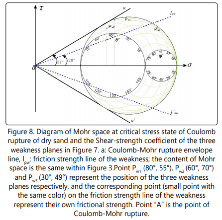
In the models, three pre-existing weakness planes (P_w1, P_w2 and P_w3), which are oblique to the extension direction (σ₃ ), with (φ´, θ´) = (80°, 55°), (60°, 70°) and (30°, 49°) respectively, are set. The weakness planes are represented by a 80mm wide slice of thin sheets of paper inserted into the base of a homogeneous layer (8.0 cm thick) of dry quartz sand (Fig. 7). Using these sheets of paper allowed localizing fault initiation, and it was easy to determine friction angle between the paper and loose sand. The friction angle of dry quartz sand is 31°, while the friction angle of sand with paper is 20° . So the µ and µ_w is 0.60 (= tg31°) and 0.36 (= tg20°). The cohesion of dry sand is very small, so C and C_w are both assumed to be equal to 0. As a result, the relative Reactivation Tendency Factor of the three weakness planes is f_a1 =1.59>f_a2 =1.42>1.0 >f_a3 =0.85 in the critical stress state of Coulomb rupture (Fig. 8), and Shear-strength Coefficient f_d1 =0.63<f_d2 = 0.70<1.0= f_a3.

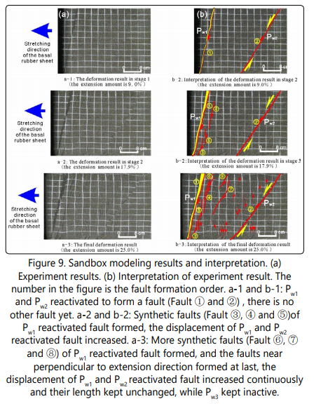
With the above model (Figure 7), the weakness, with Shear-strength Coefficient f_d1<1.0, reactivated to form several faults, one after another, in the progressive extension as predicted, and Coulomb ruptures faults form at last (Figure 9). The deformation in the progressive extension is summarized in the following:

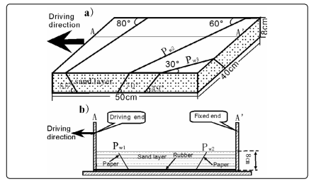
Figure 7. Experiment design of sandbox modeling. (a) Skeleton figure of experimental model. It is 40cm wide, 50cm long and 8cm thick. P_w1, P_w2, and P_w3 are weakness planes which is oriented oblique to the extension direction, with (θ´, φ´) are (80°, 55°), (60°, 70°) and (30°, 49°) respectively, and represented by paper being inserted into the homogeneous dry sand. Elastic rubber is under the sand layer and connected to driving end. (b) Section of AA´ in figure (a).

The weakness plane with the smallest Shear-strength Coefficient (P_w1) reactivated to form a fault at first (fault number 1, Fig. 9b-1). Then, the second weakness plane (P_w2) reactivated to form a fault (fault number 2, Fig. 9b-1). In the middle stage (after the weakness reactivated and before the fault near perpendicular to extension direction formed), weakness related faults which are parallel (or sub-parallel) to and controlled by P_w1 or P_w2 (antithetic and synthetic faults, fault numbers 3-8in Figures 22b-2 and b-3) began to develop near the weakness plane area. In the final stage (Fig. 9b-3), faults near perpendicular to the extension direction (small faults in Figure 9b-3) began to develop. While the third weakness plane, which Shear-strength Coefficientf_d3=1.0 (f_a3 =0.85<1.0, Fig. 8), does not reactivate as predicted. Similar experiments carried out by Tong and Yin (2011) [11] and Tong et al. (2014) [28] showed the same results.

In general, a phase of deformation indicated by the initiation of a new fault trend is attributed to a specific stress regime. However, our analysis suggests that in a region where the magnitude of differential stresses progressively increase while their directions are kept constant, multiple phases of fault initiation with different trends can occur. This could be due to reactivation of pre-existing weaknesses. The sequence of reactivation of any preexisting weakness is predictable according to the relative-orientation and mechanical properties of the weak planes.

It is not easy to estimate the shear strength of pre-existing weaknesses in the field. Even though, the relative-orientation of a weakness may be determined accurately in some circumstances (when high quality 3D seismic data is available, and fault systems in shallow level can be mapped accurately),mechanical properties of the weakness (C_w, µ_w ) are not easily determined.However, if the sequence of faulting in the geologic record is known , this information may be reversely used for assessing the mechanical properties of the preexisting weaknesses at the time of their reactivation.

Discussion

Although this study is expanding the work of Ranalli (1990) [5] and Morris et al [7], our newly defined Shearstrength Coefficient, newly developed graphical techniqueMohr-space and the underlying theoretically framework, which is based on Reactivation Tendency analysis theory (Tong and Yin, 2011), provide a much general and intuitive treatment of the shear strength decrease and anisotropies caused by pre-existing weakness(es). Specifically, the assumption that the weakness plane containing the intermediate stress (σ₂ ) in Ranalli´s (1990) [5] analysis can now be neglected. Finally, we predicted that weaknesses will reactivate sequentially according to the Shear- strength coefficient values order (from small to large) and new fractures (Coulomb rupture) form at last in the progressive deformation. It was verified by a simple sandbox experiment.

Both in this study and that of Ranalli (1990) [5], it is assumed that the preexisting weakness must be planar. This assumption, however, does not prevent the application of the analysis developed in this study to non-planar weaknesses, as curved surfaces can always be divided into approximately small planar segments. Another important assumption in our study is that fault formation, propagation and activity do not affect the regional stress distribution. This assumption is clearly an oversimplification, as both detailed analysis of faultzone evolution and regional modeling show that frictional sliding on faults is capable of creating local stress fields near the faults that are different from the regional stress field [29] [30]. However, the results of our sandbox experiment imply that the effect of activating preexisting weakness does affect local stress, but is minimal in changing regional stress. More research is clearly needed to address this problem.

Possible complex interactions between faults that lie near one another were not considered in our model. As stress concentrates at crack tips, it is expected that complex stress fields can be induced by the presence of cracks or weaknesses under uniform regional stress [30] (e.g., Gudmundsson et al., 2009). Thus, our model should be considered as an idealized conceptual guide, which can only be used in realistic situations when the above factors are considered.

Despite the complexities discussed above, our analysis does provide a new insight into the temporal evolution of multiple pre-existing weaknesses with different Shear– strength coefficient. Our analysis suggests that in a region with a progressive increase in the magnitude of differential stresses while the directions of the principal stresses are not changed, multiple phases of fault initiation with different trends can be generated. On the other hand, the results of theoretical analysis will provide some information and clues to understand actual shear strength decrease and anisotropies due to the pre-existing weaknesses.

Conclusion

Shear-strength coefficient (f_d), which is defined to evaluate the shear strength decrease due to the presence of preexistingweaknesses, is determined by the orientation and mechanical properties of weakness(the intrinsic factors) and stress tensor (the external factors), and can be calculated quantitatively. It also can be expressed intuitively/graphically in Mohr-space. The results of theoretical analysis in Mohrspace show that:

(1)Weakness relative-orientation (θ´, φ>), which is determined jointly by orientation of the weakness and three principal stress axis, is the predominant factor leading to shear strength anisotropies. (0°, φ´0 ) and (180°, φ´0 ) are two relativeorientations with the lowest f_d. As θ´ increases from 0° or decreases from 180°, and φ´ deviates from φ´0 , f_d will increase. There are critical angles φ´1 , φ´2 and θ´1 , 180°-θ´1 , when φ´1 <φ´< φ´2 or θ´1 <θ´<180°-θ´1 , f_d = 1.0. Low f_d value of weakness plane concentrates in the area around θ´=0°~15° or 165°~180° and φ´=φ´0 ± 15°.

(2)Weakness mechanical properties (C_w and µ_w) are the predominant factorsthat lead to shear strength decrease. “Discrete” weaknesses may suffer more than 80% decrease in maximum shear strength, while “pervasive” weaknesses usually suffer 20-60% decrease in maximum shear strength.

(3)The effect of relative to shear strength is a little complicated, and is related to θ´ and φ´, particularly φ´. The effect of relative σ₂ is most prominant only in the interval 40°<φ´<70°. Under normal circumstances, f_d will decrease a little with increasing of .

In a region with a progressive increase in the magnitude of differential stresses acting on multiple pre-existing weaknesses, while the directions of the principal stresses maintain the same, multiple phases of fault initiation with different trends can be generated with predicted sequence according to their shear–strength coefficient (from small to large). This theoretical prediction wasverified by the results of a sandbox model.

Acknowledgement

We would like to thank graduate students Mingyang WANG and Hua wu HAO for drawing the figures of the Mohr space and their help to complete the sandbox model.This study was supported by China National Major Project of Oil and Gas (2016ZX05024-005-004 & 2011ZX05023-004- 0122011zx05006-006-02-01) and China Natural Science Foundation (Grant No. 41272160&40772086). HAK is supported by the Swedish Research Council.

References

1. Jaeger JC. Shear fracture of anisotropic rocks. Geol. Mag. 1960; 97: 65-72.
2. Jaeger J C, Cook NGW. Fundamentals of rock mechanics (third edition): London, United Kingdom, Chapman and Hall, 1979; 593.
3. Ranalli G. Rheology of the Earth: Deformation and Flow Processes in Geophysics and Geodynamics. Allen & Unwin, London. 1987.
4. Morley C K, Haranya C, Phoosongsee WS. J Structural Geology. 2004; 26(10): 1803-29. doi: 10.1016/j.jsg.2004.02.014
5. Ranalli G, Yin ZM. Critical stress difference and orientation of faults in rocks with strength anisotropies: the two-dimensional case. J Structural Geology. 1990; 12(8): 1067-71. doi: 10.1016/0191-8141(90)90102-5
6. Morris AP, David AF, Brent H. Slip-tendency analysis and fault reactivation. Geology. 1996; 24(3): 275-78. doi: 10.1130/0091-7613
7. Morris AP, Ferrill DA. The importance of the effective intermediate principal stress (σ₂ ) to fault slip patterns. J Structural Geology. 2009; 31(9): 950-59. doi: 10.1016/j.jsg.2008.03.013
8. Spencer JE, Chase CG. Role of crustal flexure in initiation of low-angle normal faults and implications for structural evolution of the Basin and Range province. J. Geophys. Res. 1989; 94: 1765-75. doi: 10.1029/ JB094iB02p01765
9. Yin A. Origin of regional, rooted low-angle normal faults: a mechanical model and its tectonic implications. Tectonics.1989; 8(3): 469-82. doi: 10.1029/TC008i003p00469
10. Sibson RH. Frictional constraints on thrust, wrench, and normal faults. Nature. 1974; 249: 542-44. doi: 10.1038/249542a0
11. Tong H, Yin A. Reactivation tendency analysis: A theory for predicting the temporal evolution of preexisting weakness under uniform stress state. Tectonophysics. 2011; 503(3-4): 195-200. doi: 10.1016/j. tecto.2011.02.012
12. Tong HM, Wang JJ, Zhao HT, et al. Mohr space and its application to the activation prediction of pre-existing weakness. Science China: Earth Sciences. 2014; 57(7): 1-10. doi: 10.1007/s11430-014-4860-1
13. Coelho S, Passchier C. Mohr-cyclides, a 3D representation of geological tensors: The examples of stress and flow. J Structural Geology. 2008; 30(5): 580-601. doi: 10.1016/j.jsg.2008.01.003
14. Brace WF. Mohr construction in the analysis of large geological strain. Geolological Society of America Bulletin. 1961; 72(7): 1059-79. doi: 10.1130/0016-7606
15. Ramsay JG. Folding and Fracturing of Rocks. McGraw-Hill, New York 1967.
16. Delaney PT, Pollard DD, Zioney JI, MacKee EH. Field relations between dikes and joints: Emplacement processes and paleostress analysis. Journal of Geophysical Research. 1986; 91: 4920-38. doi: 10.1029/ JB091iB05p04920
17. Jolly RJH, Sanderson DJ. A Mohr circle construction for the opening of a pre-existing fracture., J Structural Geology. 1997; 19(6): 887-892. doi: 10.1016/S0191-8141(97)00014-X
18. Twiss RJ, Moores. Structural Geology. New York, W. H. Freeman and Company 1992.
19. Tong H, Cai D, Wu Y, Li X, Li X, Meng L. Activity criterion of pre-existing fabrics in non-homogeneous deformation domain. Science China (Earth Science). 2010; 53(8): 1115-25. doi: 10.1007/s11430-010-3080-6
20. Collettini C, Trippetta F. A slip tendency analysis to test mechanical and structural control on aftershock rupture planes. Earth and Planetary Science Letters. 2017; 255(3-4): 402-413. doi: 10.1016/j.epsl.2007.01.001
21. Bailey W, Ben-Zion Y. Statistics of Earthquake Stress Drops on a Heterogeneous Fault in an Elastic Half-Space. Bulletin of the Seismological Society of America. 2009; 99(3): 1786–1800.
22. Yin ZM, Ranalli G. Estimation of the frictional strength of faults from inversion of fault-slip data: a new method. J Structural Geology. 1995; 17(9): 1327-35. doi: 10.1016/0191-8141(95)00028-C
23. Wallace RE. Geometry of shearing stress and relation to faulting. J. Geol. 1951; 59: 118-130.
24. Bott MHP. The mechanics of oblique slip faulting. Geol.Mag. 1959; 96(2): 109-117.
25. McKenzie DP. The relation between fault plane solutions for earthquakes and the directions of the principal stresses. Bull.Seismol. Soc. Am. 1969; 59: 591-601.
26. Morley CK. A tectonic model for the Tertiary evolution of strike–slip faults and rift basins in SE Asia. Tectonophysics. 2002; 347(4): 189-215. doi: 10.1016/S0040-1951(02)00061-6
27. Haimson B, Rudnicki JW. The effect of the intermediate principal stress on fault formation and fault angle in siltstone. J Structural Geology. 2010; 32(11): 1701-11. doi: 10.1016/j.jsg.2009.08.017
28. Tong H, Koyi H, Huang S, Zhao H. The effect of multiple pre-existing weaknesses on formation and evolution of faults in extended sandbox models. Tectonophysics. 2014; 626: 197-212. doi: 10.1016/j. tecto.2014.04.046
29. Gudmundsson A, Simmenes TH, Larsen B, Philipp SL. Effects of internal structure and local stresses on fracture propagation, deflection, and arrest in fault zones. J. Struct. Geol. 2010; 32(11): 1643-55. doi: 10.1016/j. jsg.2009.08.013
30. Yin A. Mechanics of monoclonal systems in the Colorado plateau during the Laramide orogen. J. Geophys. Res. 1994; 99: 22043-58.