

Research Article
Hoyle's Critique of Neo-Darwinian Theory: New Evaluation Points to Possible Changes in Evolution Rates
Adjunct Professor, Department of Electrical and Computer Engineering, George Mason University, 4400 University Drive Fairfax, VA 22030 USA
*Corresponding author: Thomas B Fowler, Adjunct Professor, Department of Electrical and Computer Engineering, George Mason University, 4400 University Drive, Fairfax, VA 22030 USA, Tel: 703 993-6137, 202 316-6757, E-mail: tfowler@gmu.edu
Received: December 10, 2018 Accepted: December 15, 2018 Published: December 21, 2018
Citation: Fowler TB. Hoyle's Critique of Neo-Darwinian Theory: New Evaluation Points to Possible Changes in Evolution Rates. Madridge J Bioinform Syst Biol. 2018; 1(1): 10-18. doi: 10.18689/mjbsb-1000103
Copyright: © 2018 The Author(s). This work is licensed under a Creative Commons Attribution 4.0 International License, which permits unrestricted use, distribution, and reproduction in any medium, provided the original work is properly cited.
Abstract
Physicist and astronomer Fred Hoyle has repeatedly criticized Neo-Darwinism as a flawed theory because of mathematical and statistical problems. His comments have been used by creationists and other opponents of the theory, even though he himself did not support their views. In this paper Hoyle's critique of one aspect of Neo-Darwinism is analyzed to see what merits it may have. The conclusion is that while Hoyle's mathematics is impeccable, and thus his critique based on them has merit, he did not carry his own reasoning far enough and specifically failed to consider the possibility of large variations in selective value. This may have been due to his belief that such variations would be extremely unlikely, due to an assumption that such variations would be governed by a normal distribution. However, if a heavy-tailed distribution is involved, such variations become feasible. The net result is that evolution in its early stages may have involved large jumps, which, though infrequent, would move it along.
Keywords: Heavy-Tails; Selection; Deleterious Mutation; Rare Events; Cambrian Explosion.
Introduction
Physicist and astronomer Sir Fred Hoyle (1915-2001) was a longtime and often vehement critic of Neo-Darwinism. Since he was a reputable scientist who made many valuable contributions [1], his criticisms cannot be dismissed out of hand. Equally important, they are often used as ammunition by opponents of evolution, such as creationists, [1] who actually had N. Chandra Wickramasinghe, a colleague of Fred Hoyle, testify in a famous "Balanced Treatment" court case in Arkansas in the 1980s [2]. In this paper I will examine Hoyle's argument about the effective impossibility of evolution in asexual systems according to the paradigm envisioned by Neo-Darwinism. His critique of evolution in sexual systems is more complex and requires a much lengthier analysis that is beyond the scope of this paper. The goal of this evaluation is to determine what is of value in Hoyle's critique and what insights, if any, it can provide for the modern understanding of evolution.
We begin with Hoyle's assumptions. He starts at the beginning, with a system of asexually reproducing organisms of the simplest kind, which by all accounts would have been the first to arise and the basis for all subsequent organisms. As such, he makes the following assumptions:
Assumptions 4-6, at least, clearly do not apply today, but are presumed to be a reasonable description of the situation at the dawn of life
Darwinian evolution is often represented as an almost inevitable outcome of certain natural processes, working "like logic" in its simplicity [3]: variants arise randomly which are better than existing organisms in some respect; they are selected for, their improved genes spread through the population, and eventually enough beneficial changes occur that new species and higher taxa arise. Hoyle argues that it works "like logic" only under highly simplified (and highly unrealistic) assumptions. He builds his case with a mathematical construction of the process, and indeed the mathematics quickly do become complex and often quite counterintuitive. Essential to his analysis is an accurate view of natural selection, which is frequently misunderstood and misrepresented. The simple (and uncontroversial) fact is that the majority of mutations are deleterious, not beneficial. Natural selection does not choose the "best" in an absolute sense; it can only choose the best among an array of possibilities. Therefore even starting from a population with no defects, a number of defects must arise in order to give natural selection something on which to "bite". Since deleterious mutations occur in every generation, but beneficial mutations are few and far between, Hoyle's analysis of the problem starts with the fact of deleterious mutations and analyzes their effect on fitness and survival.
First case: no mutations
The simple case of asexual (single parent-to-child)
reproduction is the one envisioned by Darwin and which is
described in virtually all biology texts. The model employed is
that of a population in which variation exists, and natural
selection acts to stabilize the fitness level in the absence of
mutations. The mathematics is likewise simple and quite
attractive, as formalized by Hoyle [4] Assume that individuals
in a population can have one of two traits, say A and a, and
that A endows its possessors with an advantage s over those
possessing a. This advantage s is typically assumed to be
rather small, in accordance with the Darwinian and NeoDarwinian theories. Let the initial population have a fraction x
possessing trait A, and 1-x possessing trait a, and assume that
offspring are produced in the ratio 1+s: 1 by the A and a
individuals, respectively. Let pa
be the number of A's and pb
the
number of a's. Then after one generation, we will have pa
+spa
individuals with A, and pb
individuals with a, assuming (without
loss of generality) that the population of the latter is constant
from generation to generation. We are interested in how the
population of A and a individuals will change over time.
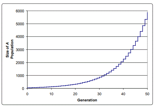
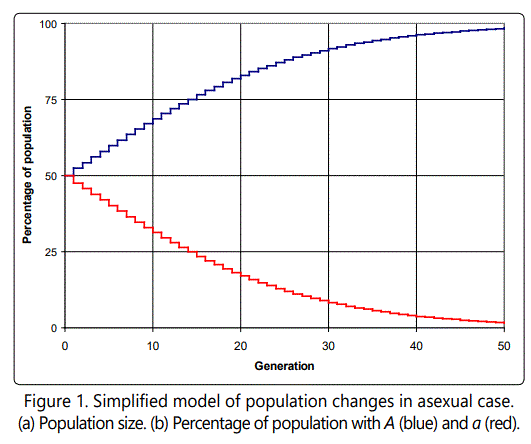
For concreteness sake, consider the following example. Assume that both A and a start with 50 individuals each in the population of 100. Let s = 0.1 (unrealistically high, but useful for this illustration). Then in the next generation, there will be 50(1+0.1) A's, and 50 a's. We can continue with further generations, repeating the calculation, and then calculate the percentage of A and a as generations (time) continue. The result is shown in Figure 1. Clearly, the selective advantage of A will cause its percentage to approach 100%, while the percentage of a's in the total population will dwindle down to near zero. In this case, the population of A's increases exponentially, as shown in Figure 1, though of course the percentage of A's in the population is limited to 100%.
To see this, note that after one generation, the change in A's is given by

As a rate of change, this becomes

In the limit as Δt approaches 0, we have
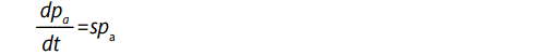
The solution to this equation may be found in any elementary calculus book as

Where pa(0) is the number of A's at time 0.
In more symbolic mathematical terms, a straightforward
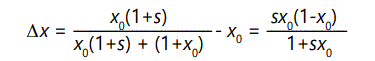
calculation shows that in the first generation, the fraction x of
A, call it x1, would increase to 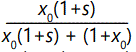 over the fraction at the beginning x0. Assuming that the number of a's remains
constant, then the change in x, δx, may be readily calculated
as
over the fraction at the beginning x0. Assuming that the number of a's remains
constant, then the change in x, δx, may be readily calculated
as
Thus the rate of increase of individuals possessing A will be
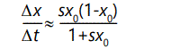
or in differential equation form,
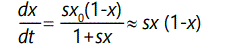
for s << 1 and assuming that change is slow and overlapping generations allow t to be approximated as a continuous variable. The solution of this equation can be readily found by using standard formulae or a computer algebra program:
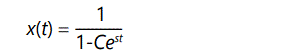
where C can be evaluated using the initial condition x=x(0) at t=0. This equation exhibits the behavior of A shown in Figure 1, above.
Note that this simple case illustrates the action of natural selection by itself, in the absence of deleterious changes or mutations; no assumption was made about the origin of the two genes A and a. They could have been part of the population's gene pool, or A could have arisen as a mutation of a.
Second (more realistic) case: errors (deleterious mutations)
Next we turn to a more realistic case which includes errors
due to mistakes in the copying process or deleterious
mutations. Ignoring for the time being the problems posed
by many-to-one and one-to-many gene mappings, consider
only the problem posed by copy errors or deleterious
mutations. This is still an oversimplified case, but will serve to
make the point. For a typical mammalian genotype,
sophisticated error correction schemes reduce the average
error rate to something on the order of 3 x 10⁻⁹. per base pair.2
With about 108
base pairs actively coding, this means that
each offspring, on average, has a chance of being miscopied
on the order of 3 x 10-9 x 108
= 0.3. We shall refer to this
average number of deleterious mutations per offspring as λ.
Such added realism causes matters to become far more
complex, and much less intuitively obvious.
To see how the scheme now works out, observe that the
number of deleterious mutations per generation will be
approximately Poisson distributed, so that the probability of k
new mutations in a particular offspring is given by
 This distribution falls off quite rapidly for values of λ less than
0.5, so we shall ignore all but the first two terms, k=0 and k=1,
i.e., 0 or 1 new mutations, with probabilities given by 1-λ and
λ, respectively, approximated to first order. We can safely
ignore the remote possibility of mutations which correct
existing defects, and as a result we are only need to consider
the cases where parents can produce offspring with the same
number or one more mutation than they themselves have. We shall further assume that each deleterious mutation reduces
the viability by the same amount, or as it is usually phrased,
each has the same adverse selection factor, call it s, assumed
negative. This means that for an individual with r mutations,
we would expect the number of offspring produced to be
reduced by (i.e., multiplied by) a factor of (1-|s|)r
as compared
to an individual with no mutations. Our goal is to determine
the average number of mutations per individual in the
population after many generations, and the corresponding
average reduction in fitness, when a steady-state condition
has been realized, assuming that all individuals of the initial or
zeroth generation have no mutations. While this is obviously
unrealistic, we do not yet know the correct answer and must
assume something to start the calculation iterations. The
value assumed for the initial generation is of no importance
as the equations will converge to the steady state value. We
shall further assume, without loss of generality, that the
population size is constant, as this will simplify our calculations.
This distribution falls off quite rapidly for values of λ less than
0.5, so we shall ignore all but the first two terms, k=0 and k=1,
i.e., 0 or 1 new mutations, with probabilities given by 1-λ and
λ, respectively, approximated to first order. We can safely
ignore the remote possibility of mutations which correct
existing defects, and as a result we are only need to consider
the cases where parents can produce offspring with the same
number or one more mutation than they themselves have. We shall further assume that each deleterious mutation reduces
the viability by the same amount, or as it is usually phrased,
each has the same adverse selection factor, call it s, assumed
negative. This means that for an individual with r mutations,
we would expect the number of offspring produced to be
reduced by (i.e., multiplied by) a factor of (1-|s|)r
as compared
to an individual with no mutations. Our goal is to determine
the average number of mutations per individual in the
population after many generations, and the corresponding
average reduction in fitness, when a steady-state condition
has been realized, assuming that all individuals of the initial or
zeroth generation have no mutations. While this is obviously
unrealistic, we do not yet know the correct answer and must
assume something to start the calculation iterations. The
value assumed for the initial generation is of no importance
as the equations will converge to the steady state value. We
shall further assume, without loss of generality, that the
population size is constant, as this will simplify our calculations.
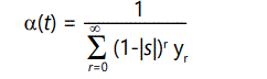
Unfortunately, to solve the problem there is no alternative to brute force enumeration and summation of all possibilities, i.e., of all offspring (k=0 or 1) from all possible parents (r=0, 1, 2,). Let yr (t) be the fraction of the population with r defects at time t. Now, an individual with r defects can produce offspring proportional to its fitness, given above as (1-|s|)r , with (1-|s|)r (1-λ) having r defects and (1-|s|)r λ having r+1 defects. However, we are assuming a stable population normalized to 1,4 so therefore the total number of offspring must sum to 1. This means that at any time t there will be a "normalizing" condition
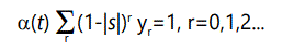
where α(t)(1-|s|)r represents the total number of offspring produced by a parent with r defects, some of which will have the same number (r) of defects as the parents, and some of which will have r+1 defects.
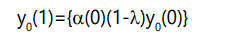
We may now set up recursion relations to determine the quantities of interest. At the first generation, the number of offspring with 0 defects will be the number produced by parents with 0 defects times the probability of zero additional defects:
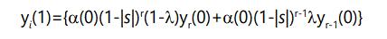
Similarly, the number of offspring with one defect will be the number of parents with 1 defect times the probability of zero additional defects, plus the number of parents with 0 defects times the probability of 1 additional defect:

In general, the number of offspring with r defects will be the number of parents with r defects times the probability of zero additional defects, plus the number of parents with r-1 defects times the probability of 1 additional defect:
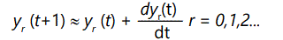
where the yi(1) terms are subject to the normalizing condition (9) above. These recursion equations can be converted to differential form by noting that
So the above equations become, in differential form,
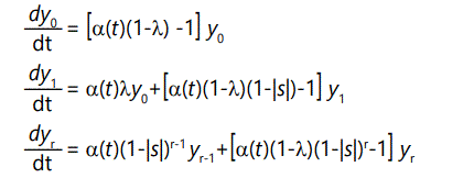
subject to normalizing condition
and boundary condition y0(0)=1; yr(0)=0, r=1,2,...
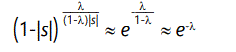
The steady-state solution to equations (14) is given to a good approximation by
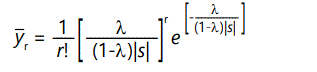
This, of course, is just the Poisson distribution with parameter (i.e. mean and variance)
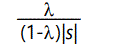
which is the average number of defects per member of the population, in the steady state, attained after approximately 4/|s| generations. The average individual, therefore, has fitness lowered by
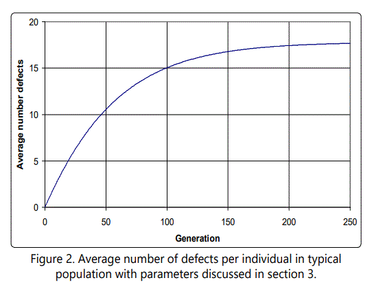
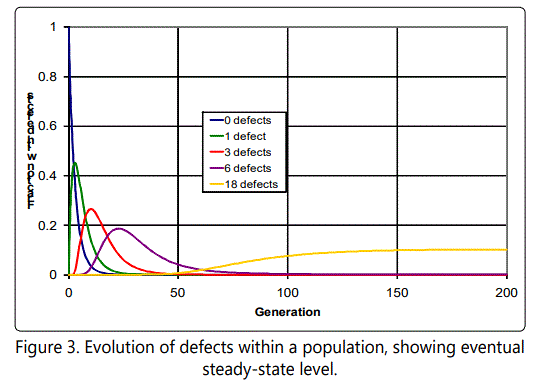
to first order in λ. To illustrate these equations and the evolution of a population which starts initially with zero defects, we consider the concrete case of l = 0.3, |s| = 0.02. This gives an expected number of defects of approximately 18, and a reduction in fitness of approximately 0.65. The number of defects as a function of generation is shown in Figure 2. The evolution of the individual yr terms, that is, the number of individuals possessing r defects, is shown in Figure 3 for several cases. Note that the population of individuals with small numbers of defects rises and then falls off, with this behavior continuing through the r values, eventually stabilizing around the expected value.
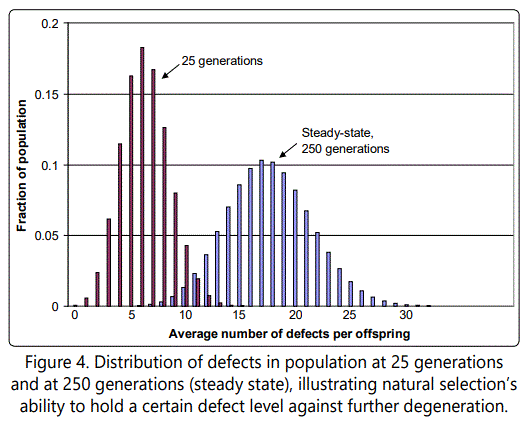
As an illustration, consider Figure 4, which shows the fraction of the population with r defects, as a function of r, in the steady-state condition. Natural selection is able to hold this distribution, i.e., prevent it from drifting further to the right. Natural selection can hold this distribution because of the higher survival rate of those with fewer mutations, which are accordingly selected for. Also shown for comparison purposes is the distribution after only 25 generations.
There are two interesting observations to be made about this case. First, note just how far we are from any sort of intuitively obvious behavior of the type envisioned by Darwin and many contemporary proponents of Neo-Darwinism; and second, observe that the mathematics has become dense and in some ways counter-intuitive, which implies that there is no substitute for rigorous analysis.
Third case: introduction of beneficial mutations
But what about beneficial mutations? Can they not still
propagate through the population as the simple model
presumes, so that the deleterious mutations are ultimately
irrelevant? Hoyle claims that this will not happen because
such beneficial mutations are completely swamped by the
deleterious mutations [4]:
When favourable mutations of the same [selection value |s|] are also considered to occur, but at a rate much less than λ, the effect is only to produce slight perturbations of the Poisson distribution [equation (16) above], perturbations that are soon stamped out under the continuing pressure of the bad mutations. Favourable mutations become swallowed in the flood of bad mutations (p. 20).
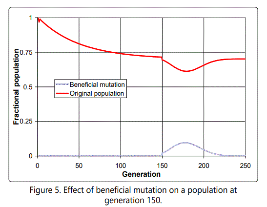
We shall see in Section 6 to what extent this conclusion is warranted. But first let us illustrate with a simple but representative case. Assume that a beneficial mutation occurs in the population discussed above, at generation 150, in an organism with 14 defects (below the average of 17). Further assume that this mutation increases fitness by a given amount, say four times the (absolute) value of the deleterious mutations; that is, this beneficial mutation is as large in the increased fitness direction as four deleterious mutations in the decreased fitness direction. As with all such cases, the exact effect of this, of course, will depend on the total population size (with a larger effect observed for a smaller population), but the results are similar. Here we have assumed a small total population of 50, so that a single organism enjoys the beneficial mutation and starts its own subpopulation, competing for resources with the rest of the non-mutated organisms. So what happens? At first the subpopulation enjoys rapid growth; but then, because it in effect starts the process of fighting the deleterious mutations afresh, they begin to grow from the starting point of 14, in effect swamping the advantages of the beneficial mutation. The effect is illustrated in Figure 5, which shows the original and mutated populations for this case. Note that up until the time of the assumed beneficial mutation, the population was stabilizing as natural selection took hold and was able to keep the number of deleterious mutations in check by differential selection of those individuals with lower numbers of defects.
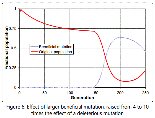
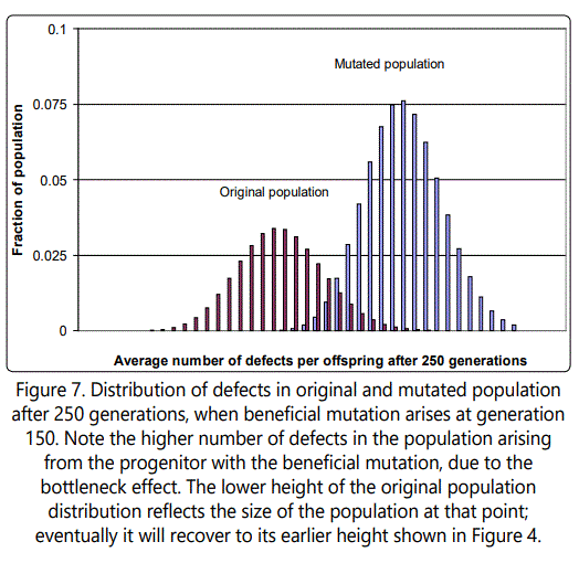
If the value of the beneficial mutation is increased further, from 4 to 10, the effect is similar, but takes longer to die out, as shown in Figure 6. Figure 7 shows the distribution of defects in the new mutated population, and illustrates the very inconvenient fact that whenever a single-parent-tooffspring population is forced to go through a single organism bottleneck (a new population arising from a single individual), as in this case, the effect is always to cause such an increase in the average number of defects, because of the need for there to be a distribution of defects among individuals on which natural selection can act, and such a distribution can only arise when the offspring of the progenitor accumulate more than it had (see Figure 8).

This result is again very counterintuitive. After all, if natural selection is selecting the most fit, why aren't the organisms with the beneficial mutation selected for? The answer is that they are, but one must consider the whole picture. In cases such as this, where a mutated line arises, it is best to think of situation as if the lines were separate species-which for all practical purposes, they are, since they do not mate and do not share genes. If there are two similar but separate species competing for the same resources, natural selection will work on them individually as well as together. That is, natural selection will select those individuals from species A that are most fit, and those from species B that are most fit. For each species, this will occur based on characteristics that they exhibit, which here are related to the number of defects each organism has (they are assumed to be identical in other respects). So each species must accumulate organisms with a range of defects, as discussed above; only then can natural selection begin its work. This will happen separately for the two species. As it occurs, natural selection will work on the overall picture-that is, the organisms from both species will be competing. If the average fitness level of one species is higher than the other after both accumulate enough of a range of defects for natural selection to operate, that species will gradually come to dominate. In the case discussed in the foregoing paragraphs, the two lines of the same organism (with and without beneficial mutation) function as separate species. That is why the organisms with the beneficial mutation do not necessarily take over the population.
Can beneficial mutations ever have an effect?
In actuality the mathematics do not absolutely prohibit
improvement by beneficial mutation, but they do constrain it
significantly, as the foregoing examples suggest. Only if a
beneficial mutation is so large that its early rapid growth can
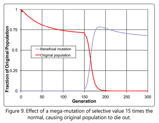
cause the original population to decline to 0 (less than 1
organism) will it take over. This case Hoyle did not consider.
Then the mutated organisms are the only ones left. This can be
seen in the previous case by increasing the selective value of
the beneficial mutation to 15, as shown in Figure 9. Thus if the
value of the beneficial mutation is sufficiently large, and the
original (unmutated) population disappears, the problems
cited above can be overcome to some degree. Curiously, such
mega-mutations are just what certain evolutionary theories
have postulated, notably those of Hugo de Vries (1848-1935)
[5], William Bateson (1868-1926) [6], and Richard Goldschmidt
(1878-1958) [7] but they were not widely accepted because of
the mathematical arguments of Sir Ronald Fisher (1890-1962)
[8, 9], namely that the assumed mechanisms of change-random genetic modifications-are always small, though this is
not a constraint imposed by physics, chemistry, or information
theory. So the bottleneck problem severely constrains the
possibilities of improvement through the mechanism of
beneficial mutations, as the defects will accumulate each time,
and soon become overpowering unless the improvement is
very large compared to the negative effects of the accumulating
defects or it occurs to a particular organism with few or no
defects (or both).
The number of beneficial mutations needed for a new species is likely to be on the order of 500. If 17 defects accumulate with each mutation, the total accumulated defects per individual would be on the order of 8,000, and obviously unsustainable number. The "mega-mutation" illustrated here is one way to escape from this "death by defect accumulation" problem, by effectively counteracting many deleterious mutations (perhaps by replacing some mechanism in the organism with a new, better one), effectively resetting the defect counter. Alternatively, it may take place in an organism which has few defects to start with, so that the defect accumulation problem is not so severe.
Hoyle did not consider this case, and concludes that the problem is insoluable without addition of sexual reproduction, which allows sharing of genes [4]:
...the usually supposed logical inevitability of the theory of evolution by natural selection [and beneficial mutations] is quite incorrect. There is no inevitability, just the reverse. It is only when the...asexual model is changed to the sophisticated model of sexual reproduction accompanied by crossover that the theory can be made to work at all, even [to a] limited degree (p. 20)
But as we have seen, this is not the only solution, even under the stated assumptions. What we can tentatively conclude from this extension of Hoyle's results are the following:
One could also argue that one or more of the original conditions (1)-(6) are incorrect, or that the parameters s (selective advantage) and/or λ (average number of mutations per offspring) are not fixed. We next consider the first of these relaxed assumptions.
Heavy tails to the rescue
The foregoing argument, based on Hoyle's text, assumes
that selective advantage s is fixed, but reveals that megamutations-those with very large selective advantage-could
be game changers. If selective advantage s is a random
variable, large values of it do indeed become possible. But
based on the usual statistical assumptions such mutations
would be exceedingly unlikely, so unlikely that they can be
dismissed as something that would never occur in the entire
lifetime of the universe. At some level this fact may have been
at the back of Hoyle's mind, though he did not discuss the
question of making s a random variable. To understand why,
take s to have a normal distribution with mean  and variance
σs2, which would be a common and reasonable assumption
given that selective advantage is the result of many factors
interacting, none of which seems to be overwhelming; and so
one can just invoke the Central Limit Theorem (CLT) as
justification. To get some feel for the degree of change this
permits, assume that s is normalized to have mean value 1,
and consider only positive values (beneficial mutations). Let
variance be given by 1. Then for a normal distribution the
probability of a beneficial mutation of value 11 (10 standard
deviations from the mean) is 3.04 x 10⁻²⁴. If there were a million
mutations per day, say in some population, the 10-sigma
event could be expected to occur about once every 3.29 x 10¹⁷
days, corresponding to about 9.01 x 10¹⁴ years-roughly 4
orders of magnitude longer than the age of universe and 5
orders of magnitude longer than the age of earth. If a megamutation of 15 standard deviations were required, the numbers
are of course far grimmer: probability of 1.046 x 10-51, which,
even at 10-12 mutations per day would still require 1.9 x 1036
years-it just won't happen, and no theory based on the need
for a large number of such occurrences can be credible.
and variance
σs2, which would be a common and reasonable assumption
given that selective advantage is the result of many factors
interacting, none of which seems to be overwhelming; and so
one can just invoke the Central Limit Theorem (CLT) as
justification. To get some feel for the degree of change this
permits, assume that s is normalized to have mean value 1,
and consider only positive values (beneficial mutations). Let
variance be given by 1. Then for a normal distribution the
probability of a beneficial mutation of value 11 (10 standard
deviations from the mean) is 3.04 x 10⁻²⁴. If there were a million
mutations per day, say in some population, the 10-sigma
event could be expected to occur about once every 3.29 x 10¹⁷
days, corresponding to about 9.01 x 10¹⁴ years-roughly 4
orders of magnitude longer than the age of universe and 5
orders of magnitude longer than the age of earth. If a megamutation of 15 standard deviations were required, the numbers
are of course far grimmer: probability of 1.046 x 10-51, which,
even at 10-12 mutations per day would still require 1.9 x 1036
years-it just won't happen, and no theory based on the need
for a large number of such occurrences can be credible.
But it could also be the case that the selective advantage s is indeed a random variable, though one which does not have a finite variance, or has a very large variance, and in some ways therefore behaves significantly differently from the normal distribution. This would occur if the probability density function of s is heavy-tailed, i.e., whose tail values fall off as a power of x rather than as e-x2 . In such case the CLT fails to apply; investigation of the reasons why it fails to apply is beyond the scope of this paper but may have to do with a special type of correlation among the variables giving rise to the selective value as demonstrated [10]. This is especially interesting because empirically heavy-tailed distributions can masquerade as normal distributions based on what would seem to be an adequate sample size [11]. However they can lead to large (far from the mean) variations, i.e., values of the random variable, which occur with much greater frequency than a normal distribution would suggest-Taleb's "black swans" appearing in genetic guise [12].
Technically, given a probability distribution function f(x), if for large x values, its cumulative distribution function F(x) has the property that it's complementary distribution

where κ1>0 and β∈[0,2], then the distribution function is said to be heavy-tailed because it falls off very slowly with increasing values of x, as shown by Willinger and Paxson [13], and Crovella and Bestavros [14]. In turn, this has an important consequence. Setting β=2 and differentiating above equation,
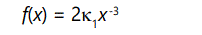
Since Var(x) = E(x2)-[E(x)]2 and [E(x)]2 is fixed, it follows that the variance is determined by
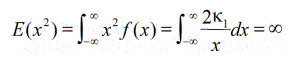
That is, the variance is infinite.
The Pareto distribution-a typical heavy-tailed distribution-has the general form
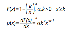
As α decreases, the "heavy-tail" effect increases. The expected value of the distribution is
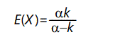
And the variance is given by
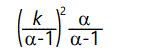
For α ≤ 1, the expected value becomes infinite. For α ≤ 2, the variance is infinite; for α > 2 the variance is finite but as a approaches 2 the variance becomes arbitrarily large. This distribution is a type of negative power law distribution, similar to the one discussed above.
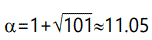
However, variance need not be infinite in this case for the desired results. Since there are two unknowns in the defining equations, a fairly straightforward calculation will yield their values for desired mean and variance. In particular, for mean and variance = 1 (same as before), the result is k=2-√2, α=1+√2 . Computing the probability of something 10 standard deviations from the mean,
For 16 standard deviations from the mean, the result is
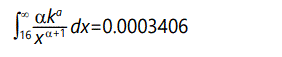
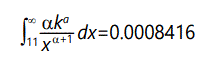
The fact that these numbers are far larger than those derived on the basis of a normal distribution suggests that the selection value is not governed by a normal distribution. In fact, these numbers are embarassingly large! It is unlikely that such large variations would be as common as these figures indicated. However this has the advantage that we can set the variance to be much less than 1 and still get "finite" values for the desired probabilities. For example, with expected value = 1, variance = 1/100, α=1+√101≈11.05 , k=(101-√101)/100≈0.9095. In this case the tail from 11 to infinity (probability of s ≥ 11) is 1.09 x 10⁻¹². In similar manner the tail from 16 to infinity (probability of s ≥ 16) is 1.73 x 10⁻¹⁴. At 1 million mutations per day, these numbers suggest about 1 megamutation (s ≥ 11) every 2500 years or every 158,000 years (s ≥ 16). Note that time for megamutations to occur is far longer than the time for populations to stabalize (~150 generations), so these will not in general affect stabilization time. Figure 11 shows these two cases of the Pareto distribution, with part of a normal distribution for comparison. Note that the narrow-variance Pareto distribution is barely distinguishable from a delta function-essentially a constant value for s.
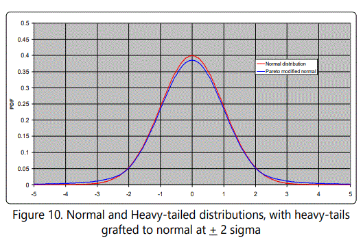
But we are actually interested in a slightly different case: the selective value of mutations can be assumed to vary continuously, with most being negative. The Pareto distribution, by itself, does not fit this bill well because it starts for x > k. It can be mirrored on the y-axis, of course, and this suggests the next step: combine positive x and negative x tails with another distribution in the middle to bridge them. This is a feasible and desirable construction because the parameters of the Pareto and Normal distributions permit joining them so that the values of the pdf and its first derivative are equal for the two distributions. The final distribution, of course, must be renormalized so that its area = 1.
A fairly straightforward calculation gives the result that
where x is expressed in units of σ, assuming without loss of generality that μ=0, since the resulting graph can be shifted to correspond to any desired value of μ. A plot is shown in Figure 10, which illustrates a normal distribution center with its usual tails and with heavy tails (Pareto distributed) grafted at ±2σ, and σ=1. Figure 11 shows the case of Pareto tails grafted at ±2σ, but with σ=0.10 and mean shifted to -1 (average selective value). This case is particularly interesting because it shows that "most" mutations would be deleterious (99.97%), and that the probability of getting a beneficial mutation of relative selective value 15 (x ≥ 16) is 8.3 x 10⁻⁸.
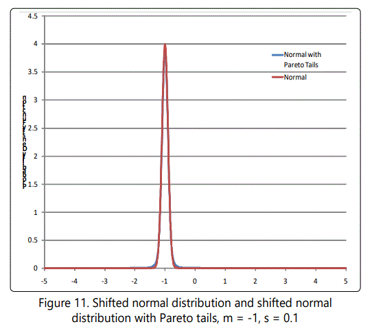
If one were taking samples, it would be difficult to distinguish these unless a large number of samples were taken. That is, "rare events" would occur, but not often enough to make an appearance in data samples. By shifting this distribution to be centered at, say, -1, the result (shown in Figure 11) can be used to make at least qualitative inferences about the hypothesis under discussion (viz. that mutations with large selective advantage can resolve Hoyle's problem).
Empirically, this would manifest itself as long periods of stasis (no beneficial megamutations) during the early period of earth's biological history (Pre-Cambrian and Cambrian), interspersed with occasional megamutations that would lead to significant organism change over very short periods. This could account for aspects of the Cambrian Explosion, when radically new developments changed the biological landscape. Thus Hoyle's results may ultimately lead to a different conclusion than he envisioned, namely that there is some truth in the large-variation theories advanced periodically to explain key aspects of evolutionary history, especially explosive change.
Results
Heavy-tailed probability distributions provide one way to resolve the problems of evolutionary change raised by Hoyle, because they make mathematically feasible large mutations that overcome the barriers Hoyle has noted. Such mutations, being rare, would appear as "jumps" and may be responsible for aspects of early history of life, such as the Cambrian Explosion. Due to the difficulties of distinguishing normal and heavy-tailed distributions using limited data sets, as well as the appeal of the Central Limit Theorem when dealing with such data, normal distributions are commonly inferred when this may not be justified. As a result, their may be a persistent bias towards estimates of selective value that are too low.
Conclusions and Future Work
Hoyle's arguments concerning the problems of evolution
in primitive systems are mathematically sound as far as they go. However, Hoyle did not consider the possibility of large
mutations, which can resolve the main problem he discusses
about the inability of such systems to evolve. He considered
the selective value of mutations to be a constant. If this
selective value is regarded as a random variable, the
probability of large mutations can be estimated. If a normal
distribution with reasonable parameters is assumed, the
probability of the large mutations is infinitesimally small.
However, if the selective value has a heavy-tailed distribution,
the situation changes dramatically. This suggests that early
organisms may have been stable for long periods, and then
made sudden large improvements-a different model than is
assumed to be operative at later times. This idea is somewhat
reminiscent of Richard Goldschmidt's "hopeful monsters"
theory [7] though based on more rigorous analysis. It is not
inconceivable that such a paradigm of organism change
underlies the Cambrian Explosion, at least in part. Future work
will model megamutation-based changes and attempt to
apply the results to periods of rapid diversification, as well as
explanation of issues in the fossil record, such as prolonged
stasis
References
Contact us for any additional information - contact@madridge.org
 Madridge Publishers is licensed under a Creative Commons Attribution 4.0 International License.