Abstract

As the use of UAVs become an essential part of human exploration across the globe, GPS scarce environments like the polar regions present a challenge for UAV navigation due to ionospheric scintillation and poor position satellite geometry making it hard to regularly obtain reliable GPS data during navigation. To overcome this challenge, this paper will evaluate and compare the use of simple dead reckoning method vs dead reckoning based on the use of inertial navigation sensor INS/GPS based on Kalman Filter for UAV navigation in the polar regions. This research paper will evaluate and compare the errors associated with the Navigation parameters position, heading using both methods while in the geographic coordinate system reference frame.

Keywords: Dead reckoning method; UAV navigation; INS/GPS Integrated System.

Abbreviations: AFDS: Autopilot Flight Director System; COG: Course Over Ground; ECEF: Earth Centered Earth Fixed; FMC: Flight Management Computer; GNSS: Global Navigation Satellite Systems; GPS: Global Positioning System; INS: Inertial Navigation System; IRU: Inertial Reference Unit; LNAV: Lateral Navigation; NED: North East Down; UAV: Unmanned Aerial Vehicle; HDG: Heading.

Introduction

Ionospheric scintillation is known as the rapid modification of radio waves. This is caused by small scale structures in the ionosphere. Severe scintillation conditions can prevent a GPS receiver from locking onto the signal and can make it impossible to calculate a position. The presence of scintillation conditions can reduce the accuracy and the confidence of positioning results. This phenomenon is frequently observed in the high latitude regions.

In these Polar Regions, the occurrence of ionospheric scintillation is largely determined by solar wind disturbances coupling to the magnetosphere–ionosphere system, resulting in steep electron density gradients and irregularities. These disturbances impact the operation of modern technology that relies on global navigation satellite systems (GNSS). Ionospheric scintillation (rapid fluctuation of radio wave amplitude and phase) degrades GPS positional accuracy and causes cycle slips, leading to a loss of lock that affects the performance of radio communication and navigation systems and thus affecting aircraft navigation in the higher latitude regions [1]. To overcome these denied GPS instances, this paper will evaluate the use of integrated INS/GPS based on Kalman Filter to complement the GPS void and compare the results with the use of simple dead reckoning. The Kalman filter is an efficient mathematical algorithm using stochastic estimation from noisy sensor measurements to produce noise reduced state outputs by using both a prediction and observational model.

INS and Use of Kalman Filter

Inertial navigation system is a self-contained navigation technique in which measurements provided by accelerometers and gyroscopes are used to track the position and orientation of an object relative to a known starting point, orientation and velocity. Inertial navigation is used in a wide range of applications including the navigation of aircraft, submarines, spacecraft and ships.

An inertial navigation system is composed of a computer and a module containing accelerometers, gyroscopes, or other motion-sensing devices. The INS is first provided with its initial position and velocity from another source like a GPS satellite receiver along with an initial heading but subsequently will update position and velocity by integrating information provided by the motion sensors. The INS advantage is that after initialization it does not requires external references to determine its position or heading.

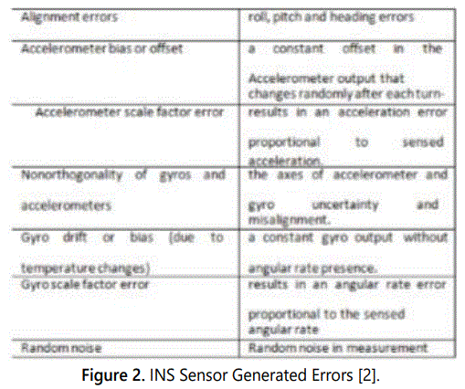
All inertial navigation systems suffer from integration drift. Small errors in the measurement of acceleration and angular velocity are integrated into progressively larger errors in velocity, which are compounded into still greater errors in position [2]. Since the new position is calculated from the previous calculated position and the measured acceleration and angular velocity, these errors accumulation are roughly proportional to the time since the initial position was input. Therefore, the position or heading must be periodically corrected by input from some other data source like GPS. Estimation theory and Kalman Filter in particular, is used to provide a theoretical framework for reducing these INS accumulated errors over time [2].

The benefits of using GPS/INS integrated in the polar regions are that the INS will be corrected by the GPS signals when available and that the INS can provide position and heading updates regularly and at faster rate whenever GPS data is not available. When GPS signal is unavailable, the INS can continue to compute the position and heading during the period of lost GPS signal. The two systems can be complementary for situations where GPS outage is more frequent.

The following statement from the Boeing Aero Magazine journal [3] accurately describes the problem: “When a North Pole (N90EXXXXX or N90WXXXXX) or South Pole (S90EXXXXX or S90WXXXXX) waypoint is used near the poles, a rapid heading and track reversal occurs as the airplane passes over the waypoint. If the airplane is operating in HDG SEL or HOLD mode while near either pole, the crew will need to rapidly update the heading selector to reflect the changing or reversed heading. Otherwise, the autopilot flight director system (AFDS) will command an unwanted turn. For autopilot operation in the polar region using a roll mode other than LNAV, the TRUE position on the heading reference switch should be selected. However, LNAV is the preferred roll mode.”

Additionally, the same Boeing technical journal [3] explains that when global positioning system (GPS) updating have timed out or are no longer valid, it is necessary to phase out all position and velocity corrections gradually until the FMC navigation parameters equal the selected IRU (Inertial reference unit) position and velocity. Also, even when GPS updates are available, they are no longer used after crossing 88.5 degrees latitude while flying toward the pole, and the crew must gradually phase out position and velocity corrections before the pole is crossed. When crossing 88 degrees latitude flying away from the pole, GPS updates are enabled, available and are considered valid [3].

INS/GPS Integration

Integrating Inertial Navigation Systems (INS) with Global Navigation Satellite System (GNSS) receivers via the Kalman filter provides better accuracy for position in high latitude navigation. This paper will investigate the combination of INS and GNSS and their integration effect in reducing UAV navigation errors and provide better accuracy, reliability and integrity than either o1ne alone.

The main component of INS is the Inertial Measurement Unit (IMU), composed of three orthogonal accelerometers and three orthogonal gyroscopes (gyros) with known relative orientation. The accelerometers provide information on linear displacement of the vehicle, whereas the gyros provide information about its angular displacement and knowing initial attitude will allow continuous calculations of the vehicleʼs attitude. Velocity and position of the vehicle are obtained through single and double integration of accelerations from accelerometers. Prior to integration, the accelerations must be transformed from the body frame of reference to the navigation frame of reference and the integrations must be initialized with the known starting velocity and position of the vehicle [4].

INS is a navigation instrument providing a complete set of information on position, velocity and angular orientation. Its main advantage is that its output data is available at a very high rate compared to GPS, making navigation continuous and responsive to rapid maneuvers of the vehicle. The main disadvantage of INS is the growing error increase over time in the absence of another sensor source to provide correction. This can result in greater position inaccuracies over time.

INS/GPS Integrated Sensor model based on Kalman Filter

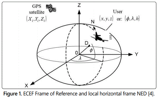
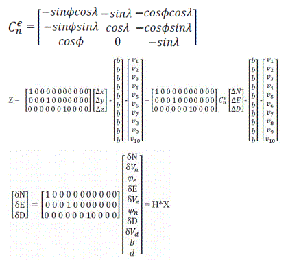
GPS satellites positions are expressed in Earth-centered Earth fixed (ECEF) Cartesian frame of reference WGS-84. The coordinates in ECEF can be presented as (x, y, z) or in geographic coordinates as latitude, longitude and height (ϕ, λ, h). GPS/INS errors will be modelled in navigation frame of reference NED (Figure 1).

The INS/GPS system has a time propagation of INS errors (Figure 2) and GPS clock errors. Modeling INS errors can be very complex and may contain even many states of complexity [4]. Most of these error states can be eliminated without affecting the INS accuracy and can be reduced to an eight-state model. The GPS receiver clock errors which are mainly bias, and drift are modeled as a 2-state random process [5,6]. The GPS receiver clock bias and drift are estimated along with other variables and their model and are used to augment the INS errors model.

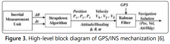
GPS is inherently a positioning system that can also derive velocity and acceleration from its code and carrier phase measurements [6]. GPS data can also be lagging or missing due to external factors like tall buildings or ionospheric scintillation. An inertial navigation system, on the other hand, senses acceleration and rotational rates and can derive position, velocity, and attitude/heading from them. INS provide very high fidelity short term dynamical information while GPS provides noisy but very stable positioning and velocity information over the long term [6]. Figure 3 below depicts a high-level block for a typical GPS/INS system. An inertial measurement unit generates acceleration (Dv) and rotation rate (Du) data at high rates typically in the range of tens or hundreds of hertz. A strapdown algorithm then accumulates these incremental measurements of Dv and Du to generate a reference trajectory consisting of position, velocity and attitude/heading with high dynamic fidelity [6]. The GPS generates data at lower rates typically one to ten hertz. These two sensors are intrinsically very complementary in nature and so the integration of these types of sensors is very much a natural fit.

Our error state system model is composed of the integration of INS and GPS. Our state space variables are made of position, velocity, attitude errors and inertial sensor biases.

The dynamics model of the INS/GPS system describes time propagation of INS errors and GPS clock errors. The input of Kalman Filter is the mixed of GPS and INS errors. After the filtering process, the random noises mostly come from GPS are removed, the remained INS errors are added to INS output to get the correct navigation value.

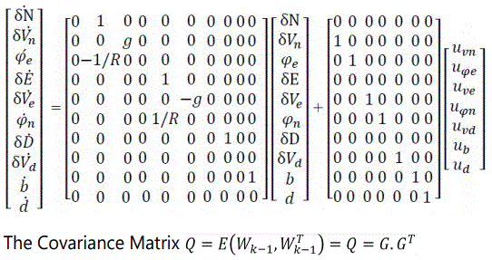
Finally, the augmented model of INS/GPS system contains 10 states, 8 for INS and 2 for GPS receiver clock. The differential equations of the GPS/INS error model propagation can be derived as follows [6]:

Let R=[ϕ, λ, h] be the UAV position in the geographic coordinates system. P=[N, E, D] the UAV position and V=[Vn, Ve, Vd] the velocity vector in the NED frame.

The INS/GPS error state vector in the ECEF frame can be expressed as : X=[δx_n, δv_n, δa_e, δx_e, δv_e, δa_n, δx_d, δv_d, b, d]^T

The INS/GPS error state vector in the NED frame can be expressed as:
X=[δN, δV_n, φ_e, δE, δV_e, φ_n, δD, δV_d, b, d ]^T
where: δN is the INS position error along the North axis [m],
δV_n - INS velocity error along the North axis [m/s],
φ_e - INS attitude error around the East axis [rad],
δE - INS position error along the East axis [m],
δV_n - INS velocity error along the East axis [m/s],
φ_n - INS attitude error around the North axis [rad],
δD - INS position error along the Down axis [m],
δV_d - INS velocity error along the Down axis [m/s],
b - GPS receiver clock bias [m],
d - GPS receiver clock drift [m/s],
Let g - gravity acceleration, R - Earthʼs radius (spherical model).

Let U be the discrete random process disturbance vector U=[u_vn, u_φe, u_ve, u_va, ub, ud]

Letʼs assume that X=[δN, δV_n, φ_e, δE, δV_e, φ_n, δD, δV_d, b, d ]^T is the initial INS/GPS error after loosing GPS. We will compare error growth of X over time with the use of Kalman Filter and without the use of the filter to evaluate the stated hypothesis below. At time t_k we will compare error X_k with X_k-1 then without the use of INS/GPS based Kalman filter.

H₀: The use of GPS/INS integrated sensor based on Kalman filter does not reduce position sensor data errors caused by polar regions ionospheric scintillation and poor satellite positioning geometry.

H₁: The use of GPS/INS integrated sensor based on Kalman filter reduces position sensor data errors caused by polar regions ionospheric scintillation and poor satellite positioning geometry.

Letʼs consider the raw data with the Kalman filter-based INS/GPS.

This consists of Integrating Inertial Navigation Systems (INS) with Global Navigation Satellite System (GNSS) receivers via the Kalman filter to see if it can reduce errors for position, velocity and attitude for UAV in navigation in the polar regions. In integrating INS with GPS, the measurement vector is composed of differences between data of the INS/GPS and the data from Kalman Filter which is the correcting system. The measurement vector contains combinations of errors of type GPS and INS. The Kalman filter does the estimates of error states, representing GPS/INS errors.

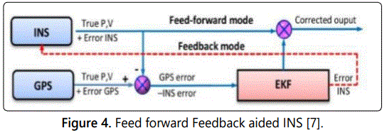
In systems consisting of feed-forward correction, increasing INS errors are estimated by Kalman Filter and subtracted from INS outputs outside of the inertial system. In INS/GNSS systems consisting of feed backward correction, the estimates of INS errors are introduced to the inertial system itself and correct its position, velocity and attitude internally (Figure 4).

In continuous time Ẋ(t) = F(t).X(t) + G(t)U(t)

where: x-state vector, u-vector of continuous random process disturbances, F-Transition matrix of the system, G-matrix of continuous process disturbances.

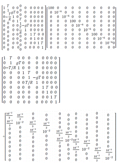
Next, we convert the continuous dynamic model to a discrete model. Then we obtain the transition matrix ϕ and the covariance matrix Q of discrete random process disturbance w defined above.

X(k+1)=ϕ(k+1,k)X(k)+w(k)

From Ẋ(t) = F(t).X(t) take the Laplace transform to get: sX(s)–x(0)=FX(s)

So, x(0)=sX(s)–FX(s)=>(sI–F)X(s)=x(0)=>X(s)=(sI–F)^-1x(0)

The inverse transform is then X(t)=L^-1(sI-F)^-1x(0) therefore ϕ=L^-1(sI-F)^-1

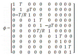
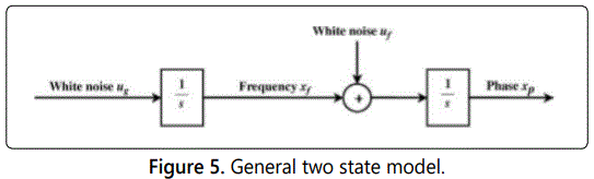
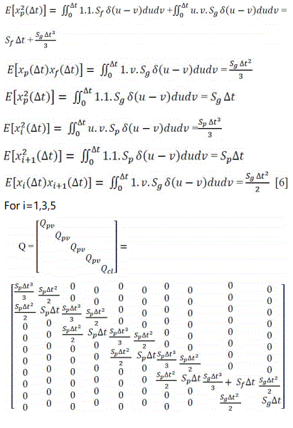
Figure 5 shows general two state model describing clock errors. The independent white noise u_f and u_g have spectral amplitudes of S_f and S_g [6].

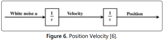
Next, we find the Q parameters of the state model following Allan variance parameters that are often used to describe clock drift [6]. We begin by writing the expressions for the variances and covariances for the general two-state model shown in figures 5 and 6. The clock states X_p and X_f represent the clock phase and frequency error, respectively. The independent white noise u_f and u_g have spectral amplitudes of S_f and S_g. Let the elapsed time since starting the white noise inputs be Δt.

Then we have:

INS/GPS Model Measurement Phase

The system provides a measurement of position and velocity, then those measurements can be obtained as

Let Z be the difference between GPS and INS position
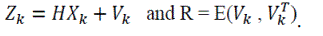
Z(t)=H(t)*X(t)+V(t) or in discrete form Z_k = H_kX_k+v_k

The INS position errors in this equation are expressed in ECEF frame of reference but the elements of state vector are expressed in NED frame (ΔN,ΔE,ΔD). We need to introduce transformation of coordinates. This can be realized by multiplying INS position errors from the state vector by the NED to ECEF coordinate transformation matrix e [5,6]

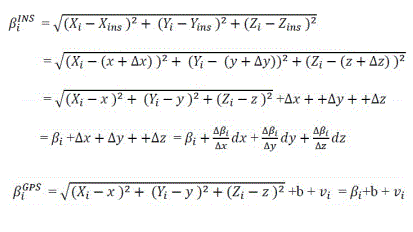
Let βi – be the UAV-satellite range from the ith satellite,
Let β_i^INS be the INS dead reckoned UAV-satellite range for i-th satellite, we will assume access to 10 satellites. Let β_i^GPS be the GPS UAV- last known satellite range for i-th satellite
Then we have the observation
z = β^INS - β^GPS = [Δβ₁, Δβ₂, Δβ₃, ......., Δβ₁₀]^T
With Δβ_i = β_i^INS- β_i^GPS

Let X_i, Y_i, Z_i - i-th satellite position, x, y, z - true UAV GPS position, and X_ins, Y_ins, Z_ins - UAV position from INS,

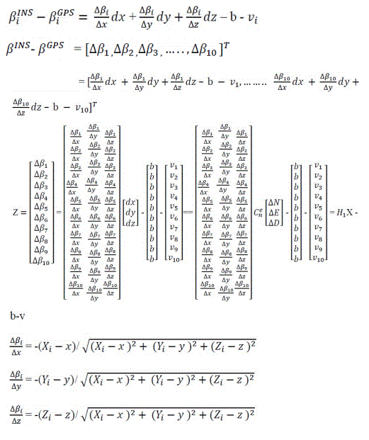
Here H=[H₁(1), 0_mx1,0_mx1, H₁(2), 0_mx1,0_mx1, H₁(3), 0_mx1,-1_mx1,0_mx1] where
H₁(i) means the i-th column of H₁ matrix

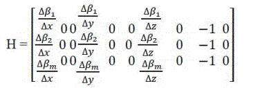
with m going up to 10

Letʼs find R the measurement error covariance matrix for V_k

They are assumed to be Gaussian zero-mean white noises of variances

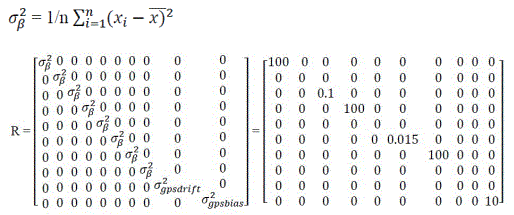
σ_a=0.10 m/s² modeled vehicle acceleration, σ_b=0.015 m/s² modeled accelerometer bias

Assume the following:
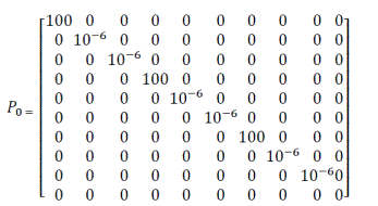
Initial position variance 10 m², initial velocity variance 0.001 m/s², initial attitude variance 0.001 rad²

Assume S_f=1.38 × 10^-4, S_g=3.54 × 10^-6, S_p=0.01 m/s²/Hz then Q is

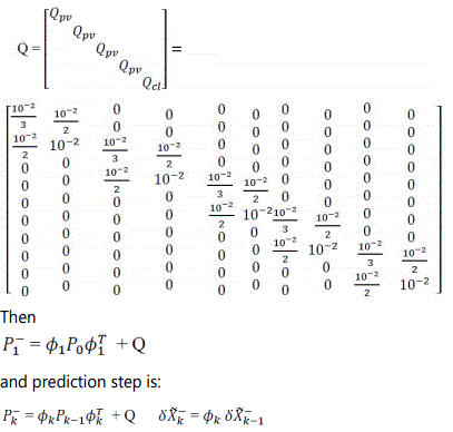
The Kalman gain is:

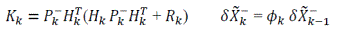
and the correction step is:

from measurement and model observation:
the pseudo range measurement is represented by: ρ=ψ+β_ρ+v_ρ
ψ=noiseless pseudo range consisting of geometric range and range error due to receiver timing error.
β_ρ=time correlated errors associated with pseudorange
v_ρ=pseudo range measurement noise [6]

The carrier phase measurement is represented by ϕ=ψ+N_ϕ+β_ϕ+ν_ϕ
N_ϕ=range uncertainty also called integer cycle ambiguity
β_ϕ=time correlated errors associated with carrier phase
ν_ϕ= carrier phase measurement noise [6]

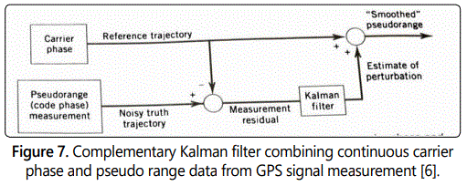
For the complimentary filter in figure 7, the carrier phase measurement representing the reference information is subtracted from the pseudo range measurement and the residual is feedback to a Kalman filter. Having extracted the observerʼs dynamics, the resulting data appears to the Kalman filter as if the modified measurement was stationary [6].

Position error model
Using the NED and ECEF coordinate transformation matrix

Simulation Data and Results

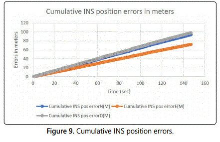
The designed integrated INS/GPS positioning system for the UAV has been tested using computer simulations. The simulations have required generation of northern latitudes trajectories for the UAVs. In this simulation GPS outage occurred in high latitude starting at position 81 N. This paper ran several simulation scenarios where the outage lasts different periods up to 40 min. A sample outage graph of 80 sec is shown in figures 8 and 9 where incremental and cumulative errors are shown.

Flight Data Position Latitude, Flight Data Position Longitude, INS position error North, INS position error East, INS position error down, Cumulative INS position error North, Cumulative INS position error East, and Cumulative INS position error East have been generated based on the Kalman filter INS/GPS calculations developed above and GPS receiver clock bias and drift as well as INS errors.

With the use of Kalman filter, the incremental positioning errors of INS decrease with the time of operation as the filter becomes more accurate in prediction, allowing slow cumulative error increase and high tolerance of loss of GPS (see figure 8). If the prediction becomes worse over time, the incremental position errors get worse causing increasing cumulative errors and low tolerance of loss of GPS.

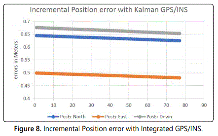
Figure 9 below shows the cumulative INS error increase in the absence of GPS with the use of Kalman filter. With the time increase, the INS cumulative errors grow and the Position Uncertainty becomes more and more unreliable. The Kalman filter allows a slow error growth as the incremental errors decrease with time (Figure 8).

Simulation of the data is shown in appendix 10 and the following output data has been collected after a simulation of several time intervals and up to 40 min: Flight Data Position Latitude, Flight Data Position Longitude, INS position error North, INS position error East, INS position error down, Cumulative INS position error North, Cumulative INS position error East, and Cumulative INS position error East. The simulation was running at a frequency of 1 and 2 Hz. Next, we plotted the cumulative INS position errors for 10 min (Figure 10) and incremental errors for a period of about 30 min (Figure 11). Figure 11 shows that after 30 min the incremental Position error values go to zero due to Correction from the Kalman filter. This simulation shows that the cumulative INS position errors grow but become bounded because the incremented position errors are decreasing with the use of the Kalman Filter.

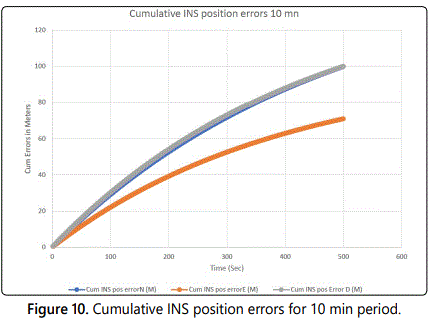
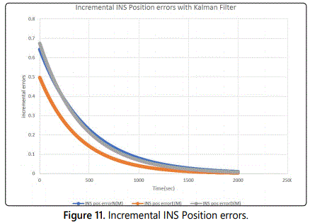
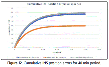
Figure 12 shows the cumulative INS errors leveling off after 30 min which is the time after which the incremental INS position errors get close to 0 as shown in figure 11.

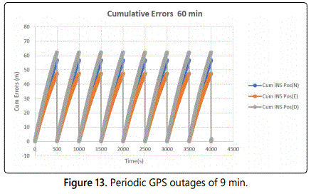
Next this paper analyzed the case of periodic GPS outage of up to 2 minutes shown in figure 13. This simulation is the case of a periodic GPS outage of 2 min i.e. losing GPS for 2 min getting it back for 1 sec and losing it again for 2 min. In this case, the cumulative position error N, E, D reset to 0 every 2 minutes due to reception of new GPS data to provide correction.

GPS Sensor without Kalman Filter

Dead reckoning is the process of calculating the UAV position by using a previously known position and advancing that position based on estimated speed, course and other variables. Dead reckoning can give very good information on position, but it is subject to errors due to speed and direction that must always be accurately known for the position to be correct. Since each estimate of position is dependent on the previous one, errors are cumulative.

The dead reckoning error model system contains 8 states. The differential equations of the error model propagation can be derived as follows:

Let R=[ϕ, λ, h] be the UAV position in the geographic coordinates system. P=[N, E, D] the UAV position and V=[Vn, Ve, Vd] the velocity vector in the NED frame.

The dead reckoning error state vector in the ECEF frame can be expressed as : X=[δx_n, δv_n, δa_e, δx_e, δv_e, δa_n, δx_d, δv_d]^T

The dead reckoning error state vector in the NED frame can be expressed as :X=[δN, δv_n, δV_n, φ_e, δE, δV_e, φ_n, δD, δV_d]^T

where: δN is the dead reckoning position error along the North axis [m],
δV_n - DR velocity error along the North axis [m/s],
φ_e - DR attitude error around the East axis [rad],
δE - DR position error along the East axis [m],
δV_e - DR velocity error along the East axis [m/s],
φ_n - DR attitude error around the North axis [rad],
δD - DR position error along the Down axis [m],
δV_d - DR velocity error along the Down axis [m/s],
Let g - gravity acceleration, R - Earthʼs radius (spherical model).

Letʼs assume that X=[δN, δv_n, δV_n, φ_e, δE, δV_e, φ_n, δD, δV_d]^T is the initial GPS error after losing GPS. We will analyze error growth of X over time without the use of the filter to evaluate the stated hypothesis on page 10. At time t_k we compared error X_k with t_k-1 without the use of Kalman filter.

In estimating the error growth of X without the use of Kalman Filter, let Δt be the dead reckoning increment time, let Crs and Hdg be the last course and heading error values due to drift since the last GPS reading.

Then δN₁=δN+sin (Hdg).δV_n.Δt, δE₁=δE+cos(Hdg).δV_e.Δt, δD₁=δD (cos(φ_n)+sin(φ_e)) δV_d. Δt/2

For the next iteration δN₂=δN₁+sin(Hdg).δV_n.Δt, δδE₂=δE₁+cos(Hdg).δV_e. Δt,
δD₂=δD(cos(φ_n)+sin(φ_e)) δV_d. Δt/2
δN₂=δN+2sin(Hdg). δV_n. Δt, δE₂=δE+2cos(Hdg). δV_e. Δt, δD₂=δD
after k iterations we have δN_k=δN+k*sin(Hdg). δV_n.Δt, δE_k=δE+k*cos(Hdg). δV_e.Δt,
δD_k=δD+k(cos(φ_n)+sin(φ_e)) δV_d. Δt

The position error growth is [k*sin (Hdg). δV_n.Δt, k*cos(Hdg).δV_e.Δt, k(cos(φ_n)+ sin(φ_e)) δV_d. Δt/2] becomes unbounded with time unlike the case of INS/GPS where the error is bounded with the use of Kalman filter (see figure 14) below. Comparing figures 12 and 14, we can see that in the dead reckoning case the cumulative position error North, East and Down is much higher and becomes quickly unbounded (Figure 14) if no GPS data is received whereas in the case of integrated INS/GPS based on Kalman filter, the position error is bounded (Figure 12). If we compare the cumulative errors at 500, 1000, 1500, 2000 and 2500 seconds we get the table 1 below.

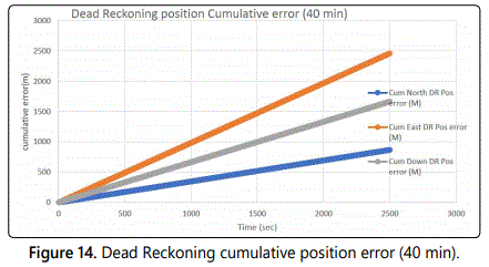
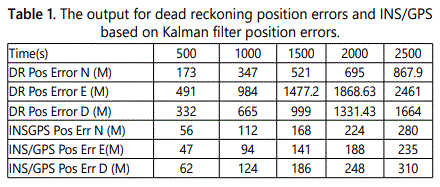
Table 1 shows the output for dead reckoning position errors and INS/GPS based on Kalman filter position errors. The variance, the mean and standard deviations are calculated for the 3 cumulative position errors. The simulation data for the integrated GPS/INS based on Kalman Filter shows that these means are 144 m, 630 m, 138 m respectively for Cumulative Position North, East and Down and 25.11, 14.93 and 27.18 for STDV and the variances of 630, 223 and 739 m. The simulation for the simple dead reckoning case shows that the means are 696, 1974 and 1335 m. These values are used to determine the Z score in high latitude position errors.

Given an error in dead reckoning position North, East and Down in the simulated data its z score is defined by z=sqrt(N)*(x-u)/ơ where u and ơ are the mean and standard deviations of position errors associated with the use of Kalman Based filter integrated INS/GPS. From the DR position errors in the simulated data, it shows that the average DR position errors North, East and Down are 696 m, 1974m, 1335m. The corresponding z scores are 406575.69, 5513920.2, 1386504 per the simulated data which leads to a probability value of 0. Recall our null and alternative hypothesis:

H₀: The use of GPS/INS integrated sensor based on Kalman filter does not reduce position sensor data errors caused by polar regions ionospheric scintillation and poor satellite positioning geometry.

H₁: The use of GPS/INS integrated sensor based on Kalman filter reduces position sensor data errors caused by polar regions ionospheric scintillation and poor satellite positioning geometry.

Letʼs consider the raw data with the Kalman filter-based INS/GPS. From our previous assumptions we assume a level of confidence C of 0.95; hence α=0.05. The critical Z score values when using a 95% confidence level are -1.96 and +1.96 standard deviations. The p-value associated with a 95% confidence level is 0.05. When the Z score is between -1.96 and +1.96, then the p-value will be greater than 0.05, and the null hypothesis cannot be rejected. Our P value will be the Probability of obtaining while in dead reckoning mode a sample with mean error equal the mean error observed in the INS/GPS integrated case with the Kalman filter assuming H0 is true; but since our P value is 0 less than α=0.05 we therefore reject the null hypothesis. Therefore, the use of GPS/INS sensor based on Kalman filter reduces sensor position data errors caused by Polar Regions ionospheric scintillation and poor satellite positioning geometry.

Conclusion

In this paper, a UAV polar navigation using INS/GPS integrated system is studied in order to compensate for the GPS denied environment limitation of UAV Polar Region operations. To model the error values, a 10-state linear Kalman Filter is implemented, and errors are evaluated comparing the INS/GPS integrated based on Kalman filter vs the simple dead reckoning case. With the INS/GPS system integrated using this configuration, itʼs possible to fly the UAV with relative high accuracy when GPS signal is integrated with INS based on Kalman filter. The data shows that in the absence of GPS, INS errors are dampened by Kalman filter to allow for position error-controlled navigation until the availability of GPS which is again used as a source of feedback for the INS. The simple dead reckoning case following GPS loss shows unbounded position errors and it is not a reliable method compared to the integrated GPS/INS. While in GPS outage mode, the integrated INS/GPS system achieved better performance using Kalman filter compared to simple dead reckoning.

References

1. Prikryl P, Ghoddousi-Fard R, Thomas EG, et al. GPS phase scintillation at high latitudes during geomagnetic storms of 7–17 March 2012 – Part 1: The North American sector. Ann Geophys. 2015; 33: 637-656. doi: 10.5194/angeo-33-637-2015   
2. Praveena K, Ravikumar A. Design of Inertial Navigation System using Kalman Filter. International Journal of Engineering Inventions. 2013; 2(12): 76-82.   
3. Boeing Commercial Airplanes. Communication and Navigation. Aero magazine Journal N 16. 2017.   
4. Kaniewski P. Aircraft positioning with INS/GNSS integrated system. Molecular and Quantum Acoustics. 2006; 27: 149-168.   
5. Salychev OS. Inertial Systems in Navigation and Geophysics. Bauman MSTU Press, Russia, 1998.   
6. Brown RG, Hwang PYC. Introduction to random signals and applied Kalman filtering: with MATLAB exercises and solutions. John Wiley & Sons, Inc., USA. 1997.   
7. Pham VT, Nguyen VT, Anh ND, Chu DT, Tran DT. 15-state extended kalman filter design for ins/gps navigation system. Journal of Automation and Control Engineering. 2015; 3(2): 109-114. doi: 10.12720/joace.3.2.109-114