Abstract

This chapter examines the relevance of errors in experimental work and discusses some basic theory necessary for an understanding of the subject. Care is taken to distinguish between the different sources of inaccuracy with the emphasis throughout being on physical understanding rather than analytical complexity.

Keywords: Analysis; Experimental studies; Systematic error; Calibration

Introduction

Experimental measurements are inevitably influenced by errors, resulting from practical limitations of the equipment, such as the minimum scale division on a pressure gauge or the high frequency cut-off behavior of an amplifier. Thus, the experimentalist must assume that errors will be present in his observations and should take the appropriate steps to minimize their influence. This requires him to be aware of the possible origins of errors and to be capable of carrying out a simple error analysis. Whilst the importance of error control cannot be emphasized too strongly, it is usually sufficient in experimental studies to perform only a simple analysis and avoid undue complexity. With a little practice, an assessment of the errors in any experiment should become a routine. The analysis should then be applied as a matter of course during the design of the experiments [1-3].

Errors in experimental work are classified into three basic categories - namely systematic errors, random errors, and “careless mistakes”.

The first two are amenable to analysis but generally require very different forms of treatment. Careless mistakes, on the other hand, are the direct responsibility of the experimenter and no amount of analysis can minimize their significance. One can only suggest caution and the incorporation of check procedures as the experiment progresses [4].

Definition of Error

Although it is easy to discuss “errors” in a qualitative manner, it is important that the meaning of this term is clearly understood before a further detailed analysis is attempted. The simplest concept of error makes use of a hypothetical true or exact value x_t which is to be compared with an individual observation x_i. By definition, the error is then given by [5]:

Clearly, the difficulty with this simple ideal will be that an exact value is rarely, if ever, available so that we must substitute an estimate of the exact value. This can be derived from a more accurate instrument, from a carefully calibrated instrument or (in the case of a system which, displays significant random behavior) by taking the arithmetic mean of a number of individual observation. That the choice has some bearing on the outcome of the error analysis should become obvious in subsequent sections [6,7].

Systematic Error

This particular kind of error leads to a constant bias in the measured values so that the data is always distorted in one direction. A typical example might be the error incurred when mercury in glass thermometer with an inaccurately drawn scale is used to measure flow temperature. In this case, repetition of the experiment will only lead to consistently wrong values with the errors always biased in the same direction at a particular temperature level even if random scatter does exist.

Elimination of systematic errors requires considerable thought before the experiment commences. Most advantageously, these errors can be eliminated by careful calibration wherever experience indicates that the accuracy of the Instrument may not be sufficient. If possible, it is advisable to use two or more quite different methods of approach to determine an experimental quantity. The presence of systematic error is then easily detected especially if calibration of one of the instruments against an accurate standard can be accomplished.

Calibration

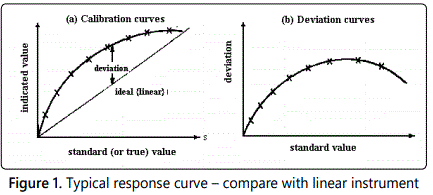
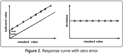
Systematic error can be detected by calibrating the instrument against an accurate standard instrument and then presenting the data in tables or, more conveniently, in graphical form. A deviation plot to show the difference between, the true value and the instrument reading. It is also useful since, it emphasizes the errors, where these might not be so obvious from the calibration curve, and therefore draws attention to those parts of the range of the instrument which are most accurate.

Ideally, an instrument would give an output signal, which varied linearly with the input signal. This linear behavior, although desirable for a number of reasons (see section 2) is not always achieved.

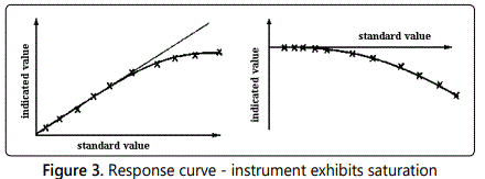
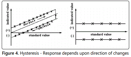
Frequently, the calibrated response curve displays one or more forms of systematic deviation from the linear relationship as illustrated in figures 1, 2, 3, 4; these deviations will be revealed if a careful static calibration of the instrument is carried out.

Other sources of systematic error can of course exist when the instrument is subjected to dynamic input signals. Whilst, in all probability, the effects of a false zero and/or nonlinearity can be corrected for under static or dynamic input conditions, the combination of hysteresis, saturation and a dynamic input signal imposes considerable problems. In this situation, the deviations become frequency dependent, i.e. systematic errors are introduced which depend upon the frequency (component) of the dynamic signal. Consideration of a typical turbulent flow property (section 6), which generally contains a range of frequencies, illustrates the difficulties thereby introduced.

The difference between the instrument reading (from the calibrated scale, perhaps) and an accurately known applied value is the systematic error. Clearly, in the extreme case where a linear calibration is assumed figure 1, then the deviation would be representative of the systematic error. Normally, however, the systematic error will be removed from the observed data using a calibration curve before the data is processed. In the first instance, when the experiment is being designed, it is nevertheless of value to examine the effect of the individual systematic errors because errors because this can reveal which quantities required special attention and care in measurement.

Additionally, a simple analysis can give some idea of the maximum possible systematic error in the final result.

Analysis of systematic errors

In most experiments, the results will be obtained by combining a number of experimentally measured quantities. If these measurements are each affected by systematic error then the result must also contain a systematic error. A simple analysis enables these errors to be related although it would obviously be better practice to remove systematic effects before calculation of the result using the calibration curves.

Systematic Errors Revealed by Calibration

Suppose a result z is evaluated from observations x, y which, have true values, x_o, y_o. Let e_x, e_y, and e_z denote the systematic errors so That:

Given a functional relationship between x, y, and z of the form:

then the systematic error e_z in the result is given to a first approximation by

Knowing the functional dependence of the result z on the measured quantities (x, y), the various systematic errors can then be related. This procedure is best explained by means of some examples.

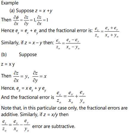
In general, systematic errors are relatively easy -to deal with once their presence has been detected by calibration. Conceptually also, they appear to cause less problems than errors resulting from random influences which require some understanding of statistical ideas.

Random Error

Statistical Treatment of Random Data

Random errors arise from the combined effects of a number of (small) fluctuating influences on the measurements. Typical sources could be changes in room temperature, the mains voltage or a mechanical vibration. Random errors are seen to be present when repetitive measurement of what is assumed to be an unchanging quantity yields values which fluctuate (in random manner) about a mean value, refer to (Figure 5). The magnitude of the random errors is assessed by using some measure of the spread of the observations about the mean value.

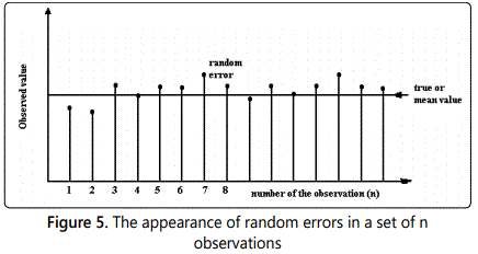
At this stage, it is possible to distinguish between the terms precise and accurate as they are applied to instrument readings. An accurate value is one which, lies consistently close to the true value and thus has negligible systematic error. In contrast, a precise instrument gives readings which, agree among themselves - having negligible scatter or RANDOM ERROR - but may nevertheless involve large systematic errors.

Thus, it is possible to obtain experimental results with high precision but poor accuracy. If the precision of the instrument is poor (significant scatter in data) then good accuracy is unlikely for a single observation but might be achieved using the mean of a large number of values.

On repeating the measurement of a random quantity, having a constant mean value and spread, it will be found that approximately equal numbers of the data lie on either side of the mean value. In fact, the mean of an infinite number of observations, which are subject only to random errors and follow a normal distribution (section 5) can be shown to equal the true value of the particular quantity. For all practical purposes, an infinite (large) number of observations are unlikely to be available usually; a small finite number of observations will be recorded instead, enabling the ‘uncertainty’ in the mean of these to be estimated using statistical analysis.

It is important to draw a clear distinction between the infinite population and; finite samples of data before any analysis of random errors is attempted. Whilst most of the theory is based on the behaviour of an infinite population, it is always the case that experimental data is in the form of a small finite sample and the theory must be modified to account for this fact.

Frequency distribution of the data before we can study random errors, we need to consider how the set of data is distributed about its mean value. There are several ways by which this spread can be described. Suppose we make repeated measurements of some quantity (typically voltage, temperature, or pressure) which is assumed to be invariant with tine. In practice, the data will be scattered about a particular level and values close to the mean will occur more often than values far from the mean.

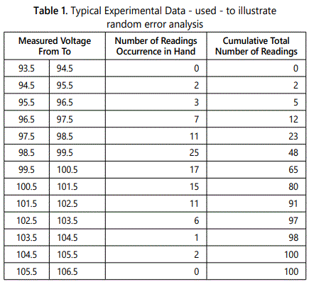
Consider, as an example, the data given in table 1 which was obtained when a nominally constant voltage was measured repeatedly using a voltmeter capable of 0.1 V resolution. The true value is known to be somewhere near 100 V and a total of 100 observations were taken. The histogram figure 6 shows how this finite sample of data can be plotted as a series of rectangles (known as a histogram) to indicate how the sample is distributed about its mean value. In this case, the width of the rectangles (1 or 2 volts) equals the width of the bands into which the data has been divided. Where the bands have equal width, the height of each rectangle represents the number of readings lying in that particular band (or range). If, for some practical reason, the bands are of unequal width, their height is determined by the condition that the area of the rectangle should be proportional to the number of observations in the band. Thus, the height of each rectangle is made proportional to (number of observations in the band/bandwidth) and the area enclosed by the histogram represents the total number of observations in the sample of data.

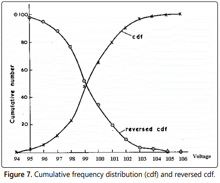
Although there is no rule for choosing the optimum number of bands into which the sample should be divided, experience shows that between five and “ten bands will generally be sufficient. The actual location and width of these bands can have a dramatic effect on the appearance of the histogram and some careful thought on the part of the experimenter is required to ensure that the wrong conclusions about the frequency distribution of the data are not reached. This is especially important where the data is to be compared with an ideal (possibly normal) distribution. In this case, it would be appropriate to make use of more sophisticated numerical descriptions of the frequency distribution rather than the shape of the histogram alone. Differences between the Normal Distribution and the sample may be expressed in terms of skewness and flatness factors as indicated in figure 7, these advanced statistical parameters are discussed by, for example, Paradine and Rivett (5).

Cumulative frequency distribution

As an alternative to the histogram, the frequency distribution of the data can be represented using a curve (or series of rectangles) to show the total number of observations occulting below a certain value. The reverse cumulative “frequency distribution curve”, showing the total number of observations occurring above a certain value could also be constructed if required. figure 7 presents the data of the previous example table 1 in these forms.

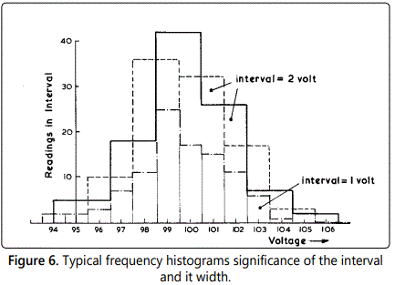
It is often more convenient to normalize both the histogram and cumulative frequency distributions so as to work in terms of percentages. Considering the histogram shown in figure 6, the proportion of the sample contained by the band centered on 99.0 volts is 0.25: this corresponds to the statement “25% of the observations lay within the range 98.5 to 99.5 voltsʼ. Recently, it has become common to employ digital computer methods to process large sets of data and thus calculate the parameters, which describe the frequency distribution and other statistical properties. [4,5] have covered this topic in considerable detail: the former in particular gives useful practical guidance on the application of these methods to fluid flow measurement.

Measures of Central Tendency

Any set of observations, which are affected by random errors, will be distributed about some mean level: this is referred to as the central tendency of the data.

To describe such a set of data, therefore, it is necessary to calculate a numerical parameter, which specifies the average value of the observations. The following two parameters are most commonly employed for this purpose.

(i)- Average value or arithmetic mean
If the observations are represented by the symbols
x₁, x₂, x₃, ...........,x_n
then the average value x̄ is defined by the expression:

(ii) Root mean square or quadratic mean value.

Although many parameters can be used to describe the amplitude of a fluctuating quantity - whether this be a time varying analogue signal or the spread of individual observations about some mean - perhaps the most familiar and useful quantity is the root mean square value. This can be defined as

in the discrete form. When a continuous analogue signal is involved, the equivalent integral expression

may be used, where “the integration time T is suitably long

Measures of Deviation from the Mean

A method, of describing how individual values are distributed about the mean value is required. The chosen parameter must take into account the frequency distribution of the data so that the percentage of observations falling within a certain range can be specified. The quantity most often chosen to describe the scatter of the data is the standard deviation defined as:

In this expression, x̄ is the mean value of the sample and x_i are the individual observations. Note the similarity of this quantity to the definition of a root mean square value given under section (2).

An alternative measure of the deviation is the variance S defined, by the expression

Infinite Population and the Normal Distribution

There is no reason in theory why the size of the sample should be restricted. Thus, it is useful to consider the ideal situation where the sample size is increased without limit and the number of observations tends to infinity (written n → ∞). In experimental work, a very common assumption is that the finite sample of data has been drawn from such an infinite sample and, moreover, that the properties of the smaller sample may be used to indicate the parameters of the infinite sample.

It can be expected that the frequency histogram and the cumulative frequency distributions would each merge into a smooth continuous curve if the size of the population were increased towards infinity and the bandwidth was simultaneously reduced to zero. Statistical analysis based on an infinite population and infinitesimally small bandwidth will enable conclusions to be drawn from the finite sample.

In situations where the measured values vary in a purely random manner, as they do in many natural processes, then the distribution of an infinitely large sample about, the mean value follows the Normal or Gaussian distribution. This idealized distribution De Moivre in 1733 states that the fraction of the total observations having a value x, or the probability of the value being x is given by the expression:

Here, σ is the standard deviation about the mean given by the integral expression

and the mean value of the infinite sample, or the population mean μ is evaluate from:

The probability p(x) is represents the chance that the particular measurement will have the value lying in the range, x to x +dx. For example, if the area under the curve between values x₁ and x₂, is 0.1, then the Normal Distribution indicated that 10% of all observations will fall within that range. Since it is theoretically possible, with an entirely random function, for any value to occur, it can be shown that:

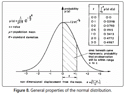
It is wrong to assume that the distribution of all variables automatically follows a Normal Distribution. Nevertheless, this ideal probability distribution often forms a good approximation to the distribution of errors in experimental data. Numerical checks are available - Paradine and Rivett (5). figure 8 shows the familiar bell-shaped curve, which represents the Normal Distribution. It has already been stated that the area beneath the curve, between specified limits, represents the probability of a measurement falling within those limits. Recognition of this figure enables the following measures of random error to be introduced.

(i) Probable Error
If the limits of μ-0.675 σ and μ + 0.675σ are considered, the area beneath the curve is found to be 0.50. Thus any observation has a 50% probability of falling within these limits. The quantity 0.675 σ sometimes referred to as the probable error in a single measurement.

(ii) Uncertainty
Choosing limits of μ - 2 σ and μ + 2 σ it can be shown that the area beneath the curve is approximately 0.95. Thus only 5% of the observations would be expected to fall outside these limits (i.e. a 20: 1 chance of exceeding this deviation from the mean value m). It is common practice to refer to the quantity ± 2 σ as the uncertainty in a single measurement.

Standard error of the mean of a sample

If we could obtain an infinite number of observations then the mean would be an accurate measurement of the quantity (provided that systematic errors were negligible). Unfortunately, it is impossible in practice to do this and we must make do with a finite sample of n observations. The mean x̄ this simple is then our best available estimate of the true population mean μ.

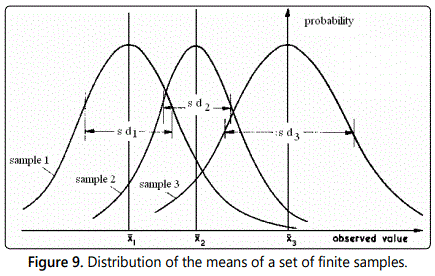
Theory shows that if we were able to measure an infinite number of such samples each that of size n from the infinite normally distributed. This normally distribution population of standard deviation s. Then the means of such samples would be distributed normally but with a smaller spread than for the population, as shown in (Figure 9). Considering the distribution of the mean values of the finite samples, then the standard deviation of this distribution is referred to as the Standard Error of the Mean (of the sample).

In a similar manner as was done for the infinite population, we can also define an Uncertainty of the Mean w_x the relationship:

Clearly, four readings will give an estimate of population mean m that will be twice as precise as an estimate based on one reading, sixteen readings will give an estimate of the mean which will be four times as precise and so on.

Before we can employ equations (6.1) and (6.2) the standard deviation of the infinite population, s must be estimated. Sampling theory shows (see Moroney (6)) that if s is the standard deviation of a finite sample of n observations then the best estimate of the population standard deviation is given by:

where, the suffix e denotes the ‘best estimate’.

The factor n/(n-1) is Besselʼs correction of the sample variance σ² to give best estimate of the population variance s² . When n is large, this factor tends to unity. Employing equations 15, 16, it therefore follows that the best estimate of the standard error of the mean is:

Similarly, we can calculate the uncertainty by of the mean simply by multiplying equation (6.4) by two.

Multi-component errors

In an experiment, it is likely that the result will depend, upon a number of measured quantities, each of which may be affected by random errors. Hence, it becomes important to calculate how these separate influences can reduce the precision of the overall result.

Where a functional relationship exists between the variables, the combined influence can be determined if the random errors in the variables are completely independent. The analysis which, follows shows how this may be achieved for the general case.

Suppose there is a relationship between the (dependent) results R and the (independent) variables x, y, z of the form:

For each variable x, y, z, R, it is possible to calculate the mean-values x̄, ȳ ,z̄ and R̄ and the random errors for each separate measurement as defined. For the purpose of this argument, denote these dx_i, dy_i, dz_i and assume that these introduce random errors in the result dR_i, where i = 1,2,3 ...,n.

Differentiation of equation (3.7.1) shows that these changes can be related, correct to first order terms, by the equation:

where the differential coefficients are to be evaluated at the mean values x̄, ȳ ,z̄ . Squaring this equation lead to:

Summing all the equations for i = 1,2,3,.......n and dividing throughout by n leads to the relationship:

Note that the cross products have an equal probability of being positive or negative (if the errors are completely random) and thus the sum of all such terms will be zero.

Reference to equation (15) shows that each term in the above equation represents the standard deviation in the particular variable: thus

With a little manipulation, this can be re-written in terms of the probable error P_R or the uncertainty w_R in the derived results R, as shown below:

Having derived these relationships, some estimate of the errors involved in each variable must be made. Since it will usually suffice to estimate the errors, rather than make an accurate calculation, even a crude estimate based on an instrument scale division or the spread displayed by a small number of repeated observations will be sufficient. A common assumption when no possibility of calculating the standard deviation of a sample exists, is to take half the minimum scale division of an instrument as an estimate uncertainty (twice the standard deviation).

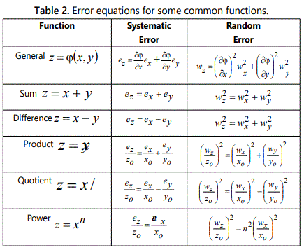
table 2 below gives expressions for the random errors associated with some typical algebraic functions. To enable a ready comparison, the calculated systematic errors are also shown alongside: the differences, which arise when dealing with the two types of error should be carefully observed.

Often, the functional relationship between, the variables will not be known, and the experiment consists of a determination of some dependent variable (R) for specified values of the independent variables (x, y, z). The only method by which the random errors can be assessed in this situation is for the observations to be repeated several times with fixed values of the independent variables, so that a scatter or tolerance band can be placed on the data. Again, the emphasis should be on making an order of magnitude estimate of the random errors, not on performing an elegant series of calculations.

For problems involving a large number of variables, this exercise can become a complicated procedure. We shall return to this topic again in the following chapters, and there consider how the uncertainties in the measured data influence the interpretation of our experimental findings.

Conclusions

The measurement of any physical quantity is inevitably influenced by experimental errors, which may be categorized as either random or systematic. The experimentalist needs to understand the difference between these two types of error and should determine which is appropriate to his own investigation before attempting an error analysis. Only relatively simple analysis is then required to determine how the Quantity will be influenced by errors in the various independent variables. This chapter has shown how calibration may be used to remove the influence of systematic errors whilst random errors can be minimized by statistical analysis.

References

1. Probert SD, Marsden JP, Holmes TV. Experimentation for students of engineering. Heinemann; 1991.   
2. Penny RK. The Experimental Method. Longman Group Limited; 1974.   
3. Lingren BW. Basic Ideas of Statistics. Macmillan; 1975.   
4. Gibson CH. Digital techniques in turbulence research. AGAK Dogapho; 1993.   
5. Paradine CE, Rivett BHP. Statistical methods for technologists. English Universities Press. 1960.   
6. Moroney MJ. Facts from figures. Penguin Press Science. 1991.   
7. Higazy MG. Experimental Measurement Theory. Cairo, CR: Dar- Elmaarifa Publisher; 2019.